Learning Objectives
- Graph systems of equations
- Graph a system of two linear equations
- Graph a system of two linear inequalities
- Evaluate ordered pairs as solutions to systems
- Determine whether an ordered pair is a solution to a system of linear equations
- Determine whether an ordered pair is a solution to a system of linear inequalities
- Classify solutions to systems
- Identify what type of solution a system will have based on its graph
The way a river flows depends on many variables including how big the river is, how much water it contains, what sorts of things are floating in the river, whether or not it is raining, and so forth. If you want to best describe its flow, you must take into account these other variables. A system of linear equations can help with that.
A system of linear equations consists of two or more linear equations made up of two or more variables such that all equations in the system are considered simultaneously. You will find systems of equations in every application of mathematics. They are a useful tool for discovering and describing how behaviors or processes are interrelated. It is rare to find, for example, a pattern of traffic flow that that is only affected by weather. Accidents, time of day, and major sporting events are just a few of the other variables that can affect the flow of traffic in a city. In this section, we will explore some basic principles for graphing and describing the intersection of two lines that make up a system of equations.
Graph a system of linear equations
In this section, we will look at systems of linear equations and inequalities in two variables. First, we will practice graphing two equations on the same set of axes, and then we will explore the different considerations you need to make when graphing two linear inequalities on the same set of axes. The same techniques are used to graph a system of linear equations as you have used to graph single linear equations. We can use tables of values, slope and y-intercept, or x– and y-intercepts to graph both lines on the same set of axes.
For example, consider the following system of linear equations in two variables.
Let’s graph these using slope-intercept form on the same set of axes. Remember that slope-intercept form looks like [latex]y=mx+b[/latex], so we will want to solve both equations for [latex]y[/latex].
First, solve for y in [latex]2x+y=-8[/latex]
[latex]\begin{array}{c}2x+y=-8\\ y=-2x - 8\end{array}[/latex]
The system is now written as
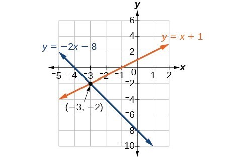
[latex]\begin{array}{c}y=-2x - 8\\y=x+1\end{array}[/latex]
Now you can graph both equations using their slopes and intercepts on the same set of axes, as seen in the figure below. Note how the graphs share one point in common. This is their point of intersection, a point that lies on both of the lines. In the next section we will verify that this point is a solution to the system.
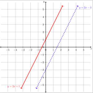
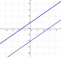
In the following example, you will be given a system to graph that consists of two parallel lines.
Example
Graph the system [latex]\begin{array}{c}y=2x+1\\y=2x-3\end{array}[/latex] using the slopes and y-intercepts of the lines.


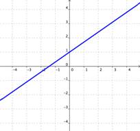
In the next example, you will be given a system whose equations look different, but after graphing, turn out to be the same line.
Example
Graph the system [latex]\begin{array}{c}y=\frac{1}{2}x+2\\2y-x=4\end{array}[/latex] using the x – and y-intercepts.

Graphing a system of linear equations consists of choosing which graphing method you want to use and drawing the graphs of both equations on the same set of axes. When you graph a system of linear inequalities on the same set of axes, there are a few more things you will need to consider.
Graph a system of two inequalities
Remember from the module on graphing that the graph of a single linear inequality splits the coordinate plane into two regions. On one side lie all the solutions to the inequality. On the other side, there are no solutions. Consider the graph of the inequality [latex]y<2x+5[/latex].
The dashed line is [latex]y=2x+5[/latex]. Every ordered pair in the shaded area below the line is a solution to [latex]y<2x+5[/latex], as all of the points below the line will make the inequality true. If you doubt that, try substituting the x and y coordinates of Points A and B into the inequality—you’ll see that they work. So, the shaded area shows all of the solutions for this inequality.
The boundary line divides the coordinate plane in half. In this case, it is shown as a dashed line as the points on the line don’t satisfy the inequality. If the inequality had been [latex]y\leq2x+5[/latex], then the boundary line would have been solid.
Let’s graph another inequality: [latex]y>−x[/latex]. You can check a couple of points to determine which side of the boundary line to shade. Checking points M and N yield true statements. So, we shade the area above the line. The line is dashed as points on the line are not true.
To create a system of inequalities, you need to graph two or more inequalities together. Let’s use [latex]y<2x+5[/latex] and [latex]y>−x[/latex] since we have already graphed each of them.
The purple area shows where the solutions of the two inequalities overlap. This area is the solution to the system of inequalities. Any point within this purple region will be true for both [latex]y>−x[/latex] and [latex]y<2x+5[/latex]. In the next example, you are given a system of two inequalities whose boundary lines are parallel to each other.
Examples
Graph the system [latex]\begin{array}{c}y\ge2x+1\\y\lt2x-3\end{array}[/latex]


In the next section, we will see that points can be solutions to systems of equations and inequalities. We will verify algebraically whether a point is a solution to a linear equation or inequality.
Determine whether an ordered pair is a solution for a system of linear equations
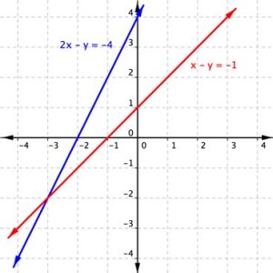
The lines in the graph above are defined as
[latex]\begin{array}{r}2x+y=-8\\ x-y=-1\end{array}[/latex].
They cross at what appears to be [latex]\left(-3,-2\right)[/latex].
Using algebra, we can verify that this shared point is actually [latex]\left(-3,-2\right)[/latex] and not [latex]\left(-2.999,-1.999\right)[/latex]. By substituting the x– and y-values of the ordered pair into the equation of each line, you can test whether the point is on both lines. If the substitution results in a true statement, then you have found a solution to the system of equations!
Since the solution of the system must be a solution to all the equations in the system, you will need to check the point in each equation. In the following example, we will substitute -3 for x and -2 for y in each equation to test whether it is actually the solution.
Example
Is [latex]\left(-3,-2\right)[/latex] a solution of the system
[latex]\begin{array}{r}2x+y=-8\\ x-y=-1\end{array}[/latex]
Example
Is (3, 9) a solution of the system
[latex]\begin{array}{r}y=3x\\2x–y=6\end{array}[/latex]
Think About It
Is [latex](−2,4)[/latex] a solution for the system
[latex]\begin{array}{r}y=2x\\3x+2y=1\end{array}[/latex]
Before you do any calculations, look at the point given and the first equation in the system. Can you predict the answer to the question without doing any algebra?
Remember that in order to be a solution to the system of equations, the values of the point must be a solution for both equations. Once you find one equation for which the point is false, you have determined that it is not a solution for the system.
We can use the same method to determine whether a point is a solution to a system of linear inequalities.
Determine whether an ordered pair is a solution to a system of linear inequalities
On the graph above, you can see that the points B and N are solutions for the system because their coordinates will make both inequalities true statements.
In contrast, points M and A both lie outside the solution region (purple). While point M is a solution for the inequality [latex]y>−x[/latex] and point A is a solution for the inequality [latex]y<2x+5[/latex], neither point is a solution for the system. The following example shows how to test a point to see whether it is a solution to a system of inequalities.
Example
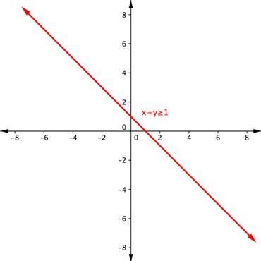
Is the point (2, 1) a solution of the system [latex]x+y>1[/latex] and [latex]2x+y<8[/latex]?
Here is a graph of the system in the example above. Notice that (2, 1) lies in the purple area, which is the overlapping area for the two inequalities.
Example
Is the point (2, 1) a solution of the system [latex]x+y>1[/latex] and [latex]3x+y<4[/latex]?
Here is a graph of this system. Notice that (2, 1) is not in the purple area, which is the overlapping area; it is a solution for one inequality (the red region), but it is not a solution for the second inequality (the blue region).
As shown above, finding the solutions of a system of inequalities can be done by graphing each inequality and identifying the region they share. Below, you are given more examples that show the entire process of defining the region of solutions on a graph for a system of two linear inequalities. The general steps are outlined below:
- Graph each inequality as a line and determine whether it will be solid or dashed
- Determine which side of each boundary line represents solutions to the inequality by testing a point on each side
- Shade the region that represents solutions for both inequalities
Example
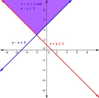
Shade the region of the graph that represents solutions for both inequalities. [latex]x+y\geq1[/latex] and [latex]y–x\geq5[/latex].


In this section we have seen that solutions to systems of linear equations and inequalities can be ordered pairs. In the next section, we will work with systems that have no solutions or infinitely many solutions.
Use a graph to classify solutions to systems
Recall that a linear equation graphs as a line, which indicates that all of the points on the line are solutions to that linear equation. There are an infinite number of solutions. As we saw in the last section, if you have a system of linear equations that intersect at one point, this point is a solution to the system. What happens if the lines never cross, as in the case of parallel lines? How would you describe the solutions to that kind of system? In this section, we will explore the three possible outcomes for solutions to a system of linear equations.
Three possible outcomes for solutions to systems of equations
Recall that the solution for a system of equations is the value or values that are true for all equations in the system. There are three possible outcomes for solutions to systems of linear equations. The graphs of equations within a system can tell you how many solutions exist for that system. Look at the images below. Each shows two lines that make up a system of equations.
| One Solution | No Solutions | Infinite Solutions |
|---|---|---|
 |
 |
 |
| If the graphs of the equations intersect, then there is one solution that is true for both equations. | If the graphs of the equations do not intersect (for example, if they are parallel), then there are no solutions that are true for both equations. | If the graphs of the equations are the same, then there are an infinite number of solutions that are true for both equations. |
- One Solution: When a system of equations intersects at an ordered pair, the system has one solution.
- Infinite Solutions: Sometimes the two equations will graph as the same line, in which case we have an infinite number of solutions.
- No Solution: When the lines that make up a system are parallel, there are no solutions because the two lines share no points in common.
Example
Using the graph of [latex]\begin{array}{r}y=x\\x+2y=6\end{array}[/latex], shown below, determine how many solutions the system has.
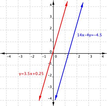
Example (Advanced)
Using the graph of [latex]\begin{array}{r}y=3.5x+0.25\\14x–4y=-4.5\end{array}[/latex], shown below, determine how many solutions the system has.
Example
How many solutions does the system [latex]\begin{array}{r}y=2x+1\\−4x+2y=2\end{array}[/latex] have?

In the next section, we will learn some algebraic methods for finding solutions to systems of equations. Recall that linear equations in one variable can have one solution, no solution, or many solutions and we can verify this algebraically. We will use the same ideas to classify solutions to systems in two variables algebraically.
Candela Citations
- Revision and Adaptation. Provided by: Lumen Learning. License: CC BY: Attribution
- Graphing a System of Linear Equation. Authored by: James Sousa (Mathispower4u.com) for Lumen Learning. Located at: https://youtu.be/BBmB3rFZLXU. License: CC BY: Attribution
- Ex 1: Graph a System of Linear Inequalities. Authored by: James Sousa (Mathispower4u.com) for Lumen Learning. Located at: https://youtu.be/ACTxJv1h2_c. License: CC BY: Attribution
- Determine if an Ordered Pair is a Solution to a System of Linear Equations. Authored by: James Sousa (Mathispower4u.com) for Lumen Learning. Located at: https://youtu.be/2IxgKgjX00k. License: CC BY: Attribution
- Determine if an Ordered Pair is a Solution to a System of Linear Inequalities. Authored by: James Sousa (Mathispower4u.com) for Lumen Learning. Located at: https://youtu.be/o9hTFJEBcXs. License: CC BY: Attribution
- Determine the Number of Solutions to a System of Linear Equations From a Graph. Authored by: James Sousa (Mathispower4u.com) for Lumen Learning. Located at: https://youtu.be/ZolxtOjcEQY. License: CC BY: Attribution
- Unit 14: Systems of Equations and Inequalities, from Developmental Math: An Open Program. Provided by: Monterey Institute of Technology and Education. Located at: http://nrocnetwork.org/resources/downloads/nroc-math-open-textbook-units-1-12-pdf-and-word-formats/. License: CC BY: Attribution