Learning Objectives
In this section, you will:
- Graph functions using stretches and compressions.
- Combine transformations.
Graphing Functions Using Stretches and Compressions
Adding a constant to the inputs or outputs of a function changed the position of a graph with respect to the axes, but it did not affect the shape of a graph. We now explore the effects of multiplying the inputs or outputs by some quantity.
We can transform the inside (input values) of a function or we can transform the outside (output values) of a function. Each change has a specific effect that can be seen graphically.
Vertical Stretches and Compressions
When we multiply a function by a positive constant, we get a function whose graph is stretched vertically away from or compressed vertically toward the x-axis in relation to the graph of the original function. If the constant is greater than 1, we get a vertical stretch; if the constant is between 0 and 1, we get a vertical compression. Figure 1 shows a function multiplied by constant factors 2 and 0.5 and the resulting vertical stretch and compression.

Figure 1 Vertical stretch and compression
Definition
Given a function [latex]f\left(x\right),[/latex] a new function [latex]g\left(x\right)=af\left(x\right),[/latex] where [latex]a[/latex] is a constant, is a vertical stretch or vertical compression of the function [latex]f\left(x\right).[/latex]
- If [latex]|a|>1,[/latex] then the graph will be stretched away from the x-axis.
- If [latex]0<|a|<1,[/latex] then the graph will be compressed toward the x-axis.
- If [latex]a<0,[/latex] then there will be combination of a vertical stretch or compression with a vertical reflection.
How To
Given a function, graph its vertical stretch or compression.
- Identify the value of [latex]a.[/latex]
- Multiply all range values by [latex]a.[/latex]
-
If [latex]|a|>1,[/latex] the graph is stretched by a factor of [latex]a.[/latex]
If [latex]0<|a|<1,[/latex] the graph is compressed by a factor of [latex]a.[/latex]
If [latex]a<0,[/latex] the graph is either stretched or compressed and also reflected about the x-axis.
Example 1: Graphing a Vertical Stretch
A function [latex]P\left(t\right)[/latex] models the population of fruit flies. The graph is shown in Figure 2.

Figure 2
A scientist is comparing this population to another population, [latex]Q,[/latex] whose growth follows the same pattern, but is twice as large. Sketch a graph of this population.

How To
Given a tabular function and assuming that the transformation is a vertical stretch or compression, create a table for the transformation.
- Determine the value of [latex]a.[/latex]
- Multiply all of the output values by [latex]a.[/latex]
Example 2: Finding a Vertical Compression of a Tabular Function
A function [latex]f[/latex] is given as Table 1. Create a table for the function [latex]g\left(x\right)=\frac{1}{2}f\left(x\right).[/latex]
| [latex]x[/latex] | 2 | 4 | 6 | 8 |
| [latex]f\left(x\right)[/latex] | 1 | 3 | 7 | 11 |
Try it #1
A function [latex]f[/latex] is given as Table 3. Create a table for the function [latex]g\left(x\right)=\frac{3}{4}f\left(x\right).[/latex]
| [latex]x[/latex] | 2 | 4 | 6 | 8 |
| [latex]f\left(x\right)[/latex] | 12 | 16 | 20 | 0 |
Example 3: Recognizing a Vertical Stretch
The graph in Figure 4 is a transformation of the toolkit function [latex]f\left(x\right)={x}^{3}.[/latex] Relate this new function [latex]g\left(x\right)[/latex] to [latex]f\left(x\right),[/latex] and then find a formula for [latex]g\left(x\right).[/latex]

Figure 4
Try it #2
Write the formula for the function that we get when we vertically stretch the identity toolkit function by a factor of 3, and then shift it down by 2 units.
Horizontal Stretches and Compressions
Now we consider the changes that occur to a function if we multiply the input of an original function [latex]f\left(x\right)[/latex] by some constant. Notice that we are changing the inside of a function. When we multiply a function’s input by a positive constant, we get a function whose graph is stretched horizontally away from or compressed horizontally toward the vertical axis in relation to the graph of the original function. If the constant is between 0 and 1, we get a horizontal stretch; if the constant is greater than 1, we get a horizontal compression of the function. Let’s consider an example.
Suppose a scientist is comparing a population of fruit flies to a population that progresses through its lifespan twice as fast as the original population. Let’s let our original population be [latex]P[/latex] and our new population be [latex]R[/latex]. Our new population, [latex]R,[/latex] will progress in 1 hour the same amount as the original population [latex]P[/latex] does in 2 hours, and in 2 hours, the new population [latex]R[/latex] will progress as much as the original population [latex]P[/latex] does in 4 hours. Sketch a graph of this population.
Symbolically, we could write
[latex]\begin{array}{l}R\left(1\right)=P\left(2\right),\hfill \\ R\left(2\right)=P\left(4\right),\text{ and in general,}\hfill \\ \text{ }R\left(t\right)=P\left(2t\right).\hfill \end{array}[/latex]
[latex]\\[/latex]
See Figure 5 for a graphical comparison of the original population and the compressed population.
![Two side-by-side graphs. The first graph has function for original population whose domain is [0,7] and range is [0,3]. The maximum value occurs at (3,3). The second graph has the same shape as the first except it is half as wide. It is a graph of transformed population, with a domain of [0, 3.5] and a range of [0,3]. The maximum occurs at (1.5, 3).](https://s3-us-west-2.amazonaws.com/courses-images/wp-content/uploads/sites/3896/2019/02/08205741/CNX_Precalc_Figure_01_05_029ab.jpg)
Figure 5 (a) Original population graph (b) Compressed population graph
Notice that the effect on the graph is a horizontal compression towards the vertical axis where all input values for our new function [latex]R[/latex] are half of the original input value for [latex]P.[/latex] You can clearly see that [latex]R\left(3\right) = P\left(6\right).[/latex] We have therefore compressed the original graph of [latex]P\left(t\right)[/latex] towards the vertical axis by a factor of ½ in order to create the graph of our new function [latex]R\left(t\right).[/latex]
Another way to think about this is that if the point (6, 2) is on the graph of [latex]P,[/latex] then the point (3, 2) will be a point on the graph of [latex]R.[/latex] We get the same outputs, but the inputs for [latex]R[/latex] are half as large as the corresponding input for [latex]P.[/latex] This results in a horizontal compression towards the vertical axis.
You should spend some time convincing yourself that if we multiplied our original input by a value between 0 and 1 that we would get a horizontal stretch away from the vertical axis. Think about what would happen if we considered another population of fruit flies who progress through their life span half as fast as those represented by [latex]P\left(t\right).[/latex] We can consider [latex]S\left(t\right) = P\left(\frac{1}{2} t\right).[/latex] This means that [latex]S\left(4\right) = P\left(2\right)[/latex] and that [latex]S\left(6\right) = P\left(3\right).[/latex] Can you see in order to get the same outputs that our inputs for the new function [latex]S[/latex] are twice as large as the inputs for the original function [latex]P?[/latex] This means there would be a horizontal stretch by a factor of 2 away from the vertical axis. Our outputs for [latex]S[/latex] are the same as the outputs for [latex]P[/latex] when the inputs for [latex]S[/latex] are double the inputs for [latex]P.[/latex] If [latex]P[/latex] has the point (3, 3) on the graph, then [latex]S[/latex] will have the point (6, 3) on the graph.
Definition
Given a function [latex]f\left(x\right),[/latex] a new function [latex]g\left(x\right)=f\left(bx\right),[/latex] where [latex]b[/latex] is a constant, is a horizontal stretch or horizontal compression of the function [latex]f\left(x\right).[/latex]
- If [latex]|b|>1,[/latex] then the graph will be compressed by a factor of [latex]\frac{1}{b}[/latex] toward the y-axis.
- If [latex]0<|b|<1,[/latex] then the graph will be stretched by a factor [latex]\frac{1}{b}[/latex] away from the y-axis.
- If [latex]b<0,[/latex] then there will be combination of a horizontal stretch or compression with a horizontal reflection.
How To
Given a description of a function, sketch a horizontal compression or stretch.
- Write a formula to represent the function.
- Set [latex]g\left(x\right)=f\left(bx\right)[/latex] where [latex]b>1[/latex] for a compression or [latex]0\lt b<1[/latex] for a stretch.
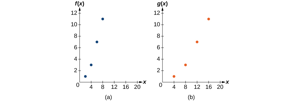
Example 4: Finding a Horizontal Stretch for a Tabular Function
A function [latex]f\left(x\right)[/latex] is given as Table 4. Create a table for the function [latex]g\left(x\right)=f\left(\frac{1}{2}x\right).[/latex]
| [latex]x[/latex] | 2 | 4 | 6 | 8 |
| [latex]f\left(x\right)[/latex] | 1 | 3 | 7 | 11 |
Example 5: Recognizing a Horizontal Compression on a Graph
Relate the function [latex]g\left(x\right)[/latex] to [latex]f\left(x\right)[/latex] in Figure 7.

Figure 7
Try it #3
Write a formula for the toolkit square root function horizontally stretched by a factor of 3.
Performing a Sequence of Transformations
When combining transformations, it is very important to consider the order of the transformations. For example, vertically shifting by 3 and then vertically stretching by a factor of 2 does not create the same graph as vertically stretching by a factor of 2 and then vertically shifting by 3, because when we shift first, both the original function and the shift get stretched, while only the original function gets stretched when we stretch first.
When we see an expression such as [latex]2f\left(x\right)+3,[/latex] which transformation should we start with? The answer here follows nicely from the order of operations. Given the output value of [latex]f\left(x\right),[/latex] we first multiply by 2, causing the vertical stretch, and then add 3, causing the vertical shift. In other words, multiplication before addition.
Horizontal transformations are a little trickier to think about. When we write [latex]g\left(x\right)=f\left(2x+3\right),[/latex] for example, we have to think about how the inputs to the function [latex]g[/latex] relate to the inputs to the function [latex]f.[/latex] Suppose we know [latex]f\left(7\right)=12.[/latex] What input to [latex]g[/latex] would produce that output? In other words, what value of [latex]x[/latex] will allow [latex]g\left(x\right)=f\left(2x+3\right)=12?[/latex] We would need [latex]2x+3=7.[/latex] To solve for [latex]x,[/latex] we would first subtract 3, resulting in a horizontal shift, and then divide by 2, causing a horizontal compression.
This format ends up being very difficult to work with, because it is usually much easier to horizontally stretch or compress a graph before shifting. We can work around this by factoring inside the function.
Let’s work through an example.
We can factor out a 2.
Now we can more clearly observe a horizontal shift to the left 2 units and a horizontal compression. Factoring in this way allows us to horizontally stretch first and then shift horizontally.
How To
Given a transformation, determine the order in which they should be preformed.
- When combining vertical transformations written in the form [latex]af\left(x\right)+k,[/latex] first vertically stretch or compress by a factor of [latex]a[/latex] and then vertically shift by [latex]k.[/latex]
- When combining horizontal transformations written in the form [latex]f\left(bx-h\right),[/latex] first horizontally shift by [latex]h[/latex] and then horizontally stretch or compress by a factor of [latex]\frac{1}{b}.[/latex]
- When combining horizontal transformations written in the form [latex]f\left(b\left(x-h\right)\right),[/latex] first horizontally stretch or compress by a factor of [latex]\frac{1}{b}[/latex] and then horizontally shift by [latex]h.[/latex]
- Horizontal and vertical transformations are independent. It does not matter whether horizontal or vertical transformations are performed first.
Example 6: Finding a Triple Transformation of a Tabular Function
Given Table 6 for the function [latex]f\left(x\right),[/latex] create a table of values for the function [latex]g\left(x\right)=2f\left(3x\right)+1.[/latex]
| [latex]x[/latex] | 6 | 12 | 18 | 24 |
| [latex]f\left(x\right)[/latex] | 10 | 14 | 15 | 17 |
Example 7: Finding a Triple Transformation of a Graph
Use the graph of [latex]f\left(x\right)[/latex] in Figure 8 to sketch a graph of [latex]k\left(x\right)=f\left(\frac{1}{2}x+1\right)-3.[/latex]

Figure 8


Example 8: Writing the Equation of a Quadratic Function from the Graph
Write an equation for the quadratic function [latex]g[/latex] in Figure 12 as a transformation of [latex]f\left(x\right)={x}^{2},[/latex]. First, write your solutions in the vertex form of a quadratic function [latex]g\left(x\right)=a{\left(x-h\right)}^{2}+k[/latex] where [latex]\left(h,\text{ }k\right)[/latex] is the vertex. Then expand the formula, and simplify terms to write the equation in general form.

Figure 12
Try it #4
A coordinate grid has been superimposed over the quadratic path of a basketball in Figure 13. Find an equation for the path of the ball. Does the shooter make the basket?

Figure 13. (credit: modification of work by Dan Meyer)
Access this online resource for additional instruction and practice with transformation of functions.
Key Equations
| Vertical shift | [latex]g\left(x\right)=f\left(x\right)+k[/latex] (up for [latex]k>0[/latex]) |
| Horizontal shift | [latex]g\left(x\right)=f\left(x-h\right)[/latex] (right for [latex]h>0[/latex]) |
| Vertical reflection | [latex]g\left(x\right)=-f\left(x\right)[/latex] |
| Horizontal reflection | [latex]g\left(x\right)=f\left(-x\right)[/latex] |
| Vertical stretch | [latex]g\left(x\right)=af\left(x\right)[/latex] ([latex]a>1[/latex] ) |
| Vertical compression | [latex]g\left(x\right)=af\left(x\right)[/latex] ([latex]0\lt a<1[/latex] ) |
| Horizontal stretch | [latex]g\left(x\right)=f\left(bx\right)[/latex] ([latex]0\lt b \lt 1[/latex] ) |
| Horizontal compression | [latex]g\left(x\right)=f\left(bx\right)[/latex] ([latex]b>1[/latex]) |
Key Concepts
- A function can be compressed or stretched vertically by multiplying the output by a constant.
- A function can be compressed or stretched horizontally by multiplying the input by a constant.
- The order in which different transformations are applied does affect the final function. Shifts and stretches must be applied in the order given. However, vertical transformations may be done before or after horizontal transformations.
Glossary
- horizontal compression
- a transformation that compresses a function’s graph horizontally, by multiplying the input by a constant [latex]b>1[/latex]
- horizontal shift
- a transformation that shifts a function’s graph left or right by adding a positive or negative constant to the input
- odd function
- a function whose graph is unchanged by combined horizontal and vertical reflection, [latex]f\left(x\right)=-f\left(-x\right),[/latex] and is symmetric about the origin
- vertical reflection
- a transformation that reflects a function’s graph across the x-axis by multiplying the output by [latex]-1[/latex]
- vertical shift
- a transformation that shifts a function’s graph up or down by adding a positive or negative constant to the output