Why Do We Care about a Normal Model?

Now we focus on the conditions for use of a normal model for the sampling distribution of differences in sample proportions.

We use a normal model for inference because we want to make probability statements without running a simulation. If we are conducting a hypothesis test, we need a P-value. If we are estimating a parameter with a confidence interval, we want to state a level of confidence. These procedures require that conditions for normality are met.

Note: If the normal model is not a good fit for the sampling distribution, we can still reason from the standard error to identify unusual values. We did this previously. For example, we said that it is unusual to see a difference of more than 4 cases of serious health problems in 100,000 if a vaccine does not affect how frequently these health problems occur. But without a normal model, we can’t say how unusual it is or state the probability of this difference occurring.

When Is a Normal Model a Good Fit for the Sampling Distribution of Differences in Proportions?

A normal model is a good fit for the sampling distribution of differences if a normal model is a good fit for both of the individual sampling distributions. More specifically, we use a normal model for the sampling distribution of differences in proportions if the following conditions are met.

[latex]{n}_{1}{p}_{1}≥10\text{ }{n}_{1}(1-{p}_{1})≥10\text{ }{n}_{2}{p}_{2}≥10\text{ }{n}_{2}(1-{p}_{2})≥10[/latex]

These conditions translate into the following statement:

The number of expected successes and failures in both samples must be at least 10. (Recall here that success doesn’t mean good and failure doesn’t mean bad. A success is just what we are counting.)

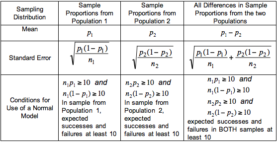
Here we complete the table to compare the individual sampling distributions for sample proportions to the sampling distribution of differences in sample proportions.

Example

More on Conditions for Use of a Normal Model

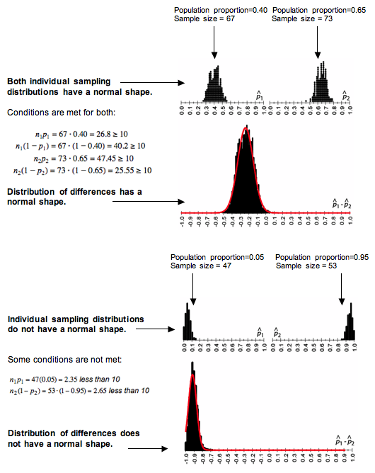
All of the conditions must be met before we use a normal model. If one or more conditions is not met, do not use a normal model. Here we illustrate how the shape of the individual sampling distributions is inherited by the sampling distribution of differences.

Using the Normal Model in Inference

When conditions allow the use of a normal model, we use the normal distribution to determine P-values when testing claims and to construct confidence intervals for a difference between two population proportions.

We can standardize the difference between sample proportions using a z-score. We calculate a z-score as we have done before.

[latex]Z\text{}=\text{}\frac{\mathrm{statistic}-\mathrm{parameter}}{\mathrm{standard}\text{}\mathrm{error}}[/latex]

For a difference in sample proportions, the z-score formula is shown below.

[latex]Z\text{}=\text{}\frac{(\mathrm{difference}\text{}\mathrm{in}\text{}\mathrm{sample}\text{}\mathrm{proportions})-(\mathrm{difference}\text{}\mathrm{in}\text{}\mathrm{population}\text{}\mathrm{proportions})}{\mathrm{standard}\text{}\mathrm{error}}[/latex]

[latex]Z\text{}=\text{}\frac{({\stackrel{ˆ}{p}}_{1}-{\stackrel{ˆ}{p}}_{2})\text{}-\text{}({p}_{1}-{p}_{2})}{\sqrt{\frac{{p}_{1}(1-{p}_{1})}{{n}_{1}}+\frac{{p}_{2}(1-{p}_{2})}{{n}_{2}}}}[/latex]

Example

Abecedarian Early Intervention Project

Recall the Abecedarian Early Intervention Project. For this example, we assume that 45% of infants with a treatment similar to the Abecedarian project will enroll in college compared to 20% in the control group. That is, we assume that a high-quality prechool experience will produce a 25% increase in college enrollment. We call this the treatment effect.

Let’s suppose a daycare center replicates the Abecedarian project with 70 infants in the treatment group and 100 in the control group. After 21 years, the daycare center finds a 15% increase in college enrollment for the treatment group. This is still an impressive difference, but it is 10% less than the effect they had hoped to see.

What can the daycare center conclude about the assumption that the Abecedarian treatment produces a 25% increase?

Previously, we answered this question using a simulation.

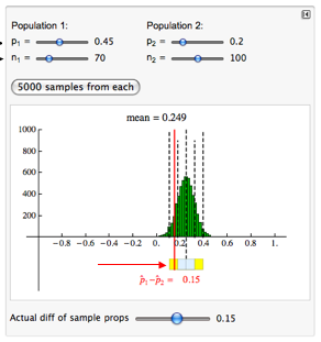
This difference in sample proportions of 0.15 is less than 2 standard errors from the mean. This result is not surprising if the treatment effect is really 25%. We cannot conclude that the Abecedarian treatment produces less than a 25% treatment effect.

Now we ask a different question: What is the probability that a daycare center with these sample sizes sees less than a 15% treatment effect with the Abecedarian treatment?

We use a normal model to estimate this probability. The simulation shows that a normal model is appropriate. We can verify it by checking the conditions. All expected counts of successes and failures are greater than 10.

For the treatment group: [latex]\begin{array}{l}70(0.45)=31.5\\ 70(0.55)=38.5\end{array}[/latex]

For the control group: [latex]\begin{array}{l}100(0.20)=20\\ 100(0.80)=80\end{array}[/latex]

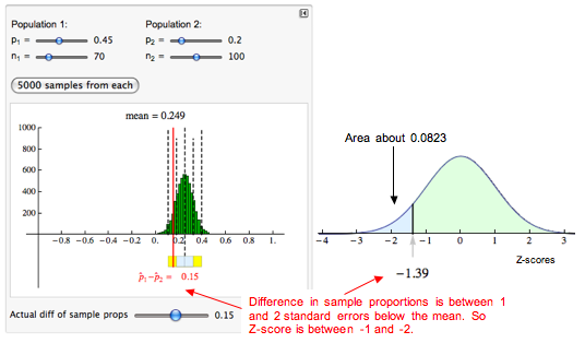
In the simulated sampling distribution, we can see that the difference in sample proportions is between 1 and 2 standard errors below the mean. So the z-score is between −1 and −2. When we calculate the z-score, we get approximately −1.39.

[latex]Z=\frac{(\mathrm{difference}\text{}\mathrm{in}\text{}\mathrm{sample}\text{}\mathrm{proportions})\text{}-\text{}(\mathrm{difference}\text{}\mathrm{in}\text{}\mathrm{population}\text{}\mathrm{proportions})}{\mathrm{standard}\text{}\mathrm{error}}[/latex]

[latex]\mathrm{standard}\text{}\mathrm{error}\text{}=\text{}\sqrt{\frac{0.45(0.55)}{70}+\frac{0.20(0.80)}{100}}\text{}\approx \text{}0.072[/latex]

[latex]Z\text{}=\text{}\frac{0.15-0.25}{0.072}\text{}\approx \text{}-1.39[/latex]

We use a simulation of the standard normal curve to find the probability. We get about 0.0823.

Conclusion: If there is a 25% treatment effect with the Abecedarian treatment, then about 8% of the time we will see a treatment effect of less than 15%. This probability is based on random samples of 70 in the treatment group and 100 in the control group.

Let’s Summarize

In “Distributions of Differences in Sample Proportions,” we compared two population proportions by subtracting. When we select independent random samples from the two populations, the sampling distribution of the difference between two sample proportions has the following shape, center, and spread.

Shape:

A normal model is a good fit for the sampling distribution if the number of expected successes and failures in each sample are all at least 10. Written as formulas, the conditions are as follows.

[latex]{n}_{1}{p}_{1}≥10\text{ }{n}_{1}(1-{p}_{1})≥10\text{ }{n}_{2}{p}_{2}≥10\text{ }{n}_{2}(1-{p}_{2})≥10[/latex]

Center:

Regardless of shape, the mean of the distribution of sample differences is the difference between the population proportions, [latex]{p}_{1}-{p}_{2}[/latex] . This is always true if we look at the long-run behavior of the differences in sample proportions.

Spread:

As we know, larger samples have less variability. The formula for the standard error is related to the formula for standard errors of the individual sampling distributions that we studied in Linking Probability to Statistical Inference.

[latex]\sqrt{\frac{{p}_{1}(1-{p}_{1})}{{n}_{1}}+\frac{{p}_{2}(1-{p}_{2})}{{n}_{2}}}[/latex]

If a normal model is a good fit, we can calculate z-scores and find probabilities as we did in Modules 6, 7, and 8. The formula for the z-score is similar to the formulas for z-scores we learned previously.

[latex]\begin{array}{l}Z\text{}=\text{}\frac{\mathrm{statistic}-\mathrm{parameter}}{\mathrm{standard}\text{}\mathrm{error}}\\ Z\text{}=\text{}\frac{(\mathrm{difference}\text{}\mathrm{in}\text{}\mathrm{sample}\text{}\mathrm{proportions})-(\mathrm{difference}\text{}\mathrm{in}\text{}\mathrm{population}\text{}\mathrm{proportions})}{\mathrm{standard}\text{}\mathrm{error}}\\ Z\text{}=\text{}\frac{({\stackrel{ˆ}{p}}_{1}-{\stackrel{ˆ}{p}}_{2})\text{}-\text{}({p}_{1}-{p}_{2})}{\sqrt{\frac{{p}_{1}(1-{p}_{1})}{{n}_{1}}+\frac{{p}_{2}(1-{p}_{2})}{{n}_{2}}}}\end{array}[/latex]