Learning Objectives
- Conduct a chi-square test of homogeneity. Interpret the conclusion in context.
We have learned the details for two chi-square tests, the goodness-of-fit test, and the test of independence. Now we focus on the third and last chi-square test that we will learn, the test for homogeneity. This test determines if two or more populations (or subgroups of a population) have the same distribution of a single categorical variable.
The test of homogeneity expands the test for a difference in two population proportions, which is the two-proportion Z-test we learned in Inference for Two Proportions. We use the two-proportion Z-test when the response variable has only two outcome categories and we are comparing two populations (or two subgroups.) We use the test of homogeneity if the response variable has two or more categories and we wish to compare two or more populations (or subgroups.)
We can answer the following research questions with a chi-square test of homogeneity:
- Does the use of steroids in collegiate athletics differ across the three NCAA divisions?
- Was the distribution of political views (liberal, moderate, conservative) different for last three presidential elections in the United States?
The null hypothesis states that the distribution of the categorical variable is the same for the populations (or subgroups). In other words, the proportion with a given response is the same in all of the populations, and this is true for all response categories. The alternative hypothesis says that the distributions differ.
Note: Homogeneous means the same in structure or composition. This test gets its name from the null hypothesis, where we claim that the distribution of the responses are the same (homogeneous) across groups.
To test our hypotheses, we select a random sample from each population and gather data on one categorical variable. As with all chi-square tests, the expected counts reflect the null hypothesis. We must determine what we expect to see in each sample if the distributions are identical. As before, the chi-square test statistic measures the amount that the observed counts in the samples deviate from the expected counts.
Example
Steroid Use in Collegiate Sports
In 2006, the NCAA published a report called “Substance Use: NCAA Study of Substance Use of College Student-Athletes.” We use data from this report to investigate the following question: Does steroid use by student athletes differ for the three NCAA divisions?
The data comes from a random selection of teams in each NCAA division. The sampling plan was somewhat complex, but we can view the data as though it came from a random sample of athletes in each division. The surveys are anonymous to encourage truthful responses.
To see the NCAA report on substance use, click here.
Step 1: State the hypotheses.
In the test of homogeneity, the null hypothesis says that the distribution of a categorical response variable is the same in each population. In this example, the categorical response variable is steroid use (yes or no). The populations are the three NCAA divisions.
- H0: The proportion of athletes using steroids is the same in each of the three NCAA divisions.
- Ha: The proportion of athletes using steroids is not same in each of the three NCAA divisions.
Note: These hypotheses imply that the proportion of athletes not using steroids is also the same in each of the three NCAA divisions, so we don’t need to state this explicitly. For example, if 2% of the athletes in each division are using steroids, then 98% are not.
Here is an alternative way we could state the hypotheses for a test of homogeneity.
- H0: For each of the three NCAA divisions, the distribution of “yes” and “no” responses to the question about steroid use is the same.
- Ha: The distribution of responses is not the same.
Step 2: Collect and analyze the data.
We summarized the data from these three samples in a two-way table.

We use percentages to compare the distributions of yes and no responses in the three samples. This step is similar to our data analysis for the test of independence.
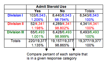
We can see that Division I and Division II schools have essentially the same percentage of athletes who admit steroid use (about 1.2%). Not surprisingly, the least competitive division, Division III, has a slightly lower percentage (about 1.0%). Do these results suggest that the proportion of athletes using steroids is the same for the three divisions? Or is the difference seen in the sample of Division III schools large enough to suggest differences in the divisions? After all, the sample sizes are very large. We know that for large samples, a small difference can be statistically significant. Of course, we have to conduct the test of homogeneity to find out.
Note: We decided not to use ribbon charts for visual comparison of the three distributions because the percentage admitting steroid use is too small in each sample to be visible.
Step 3: Assess the evidence.
We need to determine the expected values and the chi-square test statistic so that we can find the P-value.
Calculating Expected Values for a Test of Homogeneity
Expected counts always describe what we expect to see in a sample if the null hypothesis is true. In this situation, we expect the percentage using steroids to be the same for each division. What percentage do we use? We find the percentage using steroids in the combined samples. This calculation is the same as we did when finding expected counts for a test of independence, though the logic of the calculation is subtly different.
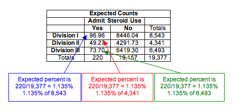
Here are the calculations for the response “yes”:
- Percentage using steroids in combined samples: 220/19,377 = 0.01135 = 1.135%
Expected count of steroid users for Division I is 1.135% of Division I sample:
- 0.01135(8,543) = 96.96
Expected count of steroid users for Division II is 1.135% of Division II sample:
- 0.01135(4,341) = 49.27
Expected count of steroid users for Division III is 1.135% of Division III sample:
- 0.01135(6,493) = 73.70
Checking Conditions
The conditions for use of the chi-square distribution are the same as we learned previously:
- A sample is randomly selected from each population.
- All of the expected counts are 5 or greater.
Since this data meets the conditions, we can proceed with calculating the χ2 test statistic.
Calculating the Chi-Square Test Statistic
There are no changes in the way we calculate the chi-square test statistic.
[latex]{\chi }^{2}\text{}=\text{}∑\frac{{(\mathrm{observed}-\mathrm{expected})}^{2}}{\mathrm{expected}}[/latex]
We use technology to calculate the chi-square value. For this example, we show the calculation. There are six terms, one for each cell in the 3 × 2 table. (We ignore the totals, as always.)

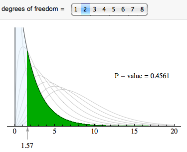
Finding Degrees of Freedom and the P-Value
For chi-square tests based on two-way tables (both the test of independence and the test of homogeneity), the degrees of freedom are (r − 1)(c − 1), where r is the number of rows and c is the number of columns in the two-way table (not counting row and column totals). In this case, the degrees of freedom are (3 − 1)(2 − 1) = 2.
We use the chi-square distribution with df = 2 to find the P-value. The P-value is large (0.4561), so we fail to reject the null hypothesis.
Step 4: Conclusion.
The data does not provide strong enough evidence to conclude that steroid use differs in the three NCAA divisions (P-value = 0.4561).
Learn By Doing
First Use of Anabolic Steroids by NCAA Athletes
The NCAA survey includes this question: “When, if ever, did you start using anabolic steroids?” The response options are: have never used, before junior high, junior high, high school, freshman year of college, after freshman year of college. We focused on those who admitted use of steroids and compared the distribution of their responses for the years 1997, 2001, and 2005. (These are the years that the NCAA conducted the survey. Counts are estimates from reported percentages and sample size.) Recall that the NCAA uses random sampling in its sampling design.

Please click here to open the simulation for use in the following activity.
We now know the details for the chi-square test for homogeneity. We conclude with two activities that will give you practice recognizing when to use this test.
Learn By Doing
Gender and Politics
Consider these two situations:
- A: Liberal, moderate, or conservative: Are there differences in political views of men and women in the United States? We survey a random sample of 100 U.S. men and 100 U.S. women.
- B: Do you plan to vote in the next presidential election? We ask a random sample of 100 U.S. men and 100 U.S. women. We look for differences in the proportion of men and women planning to vote.
Learn By Doing
Steroid Use for Male Athletes in NCAA Sports
We plan to compare steroid use for male athletes in NCAA baseball, basketball, and football. We design two different sampling plans.
- A: Survey distinct random samples of NCAA athletes from each sport: 500 baseball players, 400 basketball players, 900 football players.
- B. Survey a random sample of 1,800 NCAA male athletes and categorize players by sport and admitted steroid use. Responses are anonymous.
Let’s Summarize
In “Chi-Square Tests for Two-Way Tables,” we discussed two different hypothesis tests using the chi-square test statistic:
- Test of independence for a two-way table
- Test of homogeneity for a two-way table
Test of Independence for a Two-Way Table
- In the test of independence, we consider one population and two categorical variables.
- In Probability and Probability Distribution, we learned that two events are independent if P(A|B) = P(A), but we did not pay attention to variability in the sample. With the chi-square test of independence, we have a method for deciding whether our observed P(A|B) is “too far” from our observed P(A) to infer independence in the population.
- The null hypothesis says the two variables are independent (or not associated). The alternative hypothesis says the two variables are dependent (or associated).
- To test our hypotheses, we select a single random sample and gather data for two different categorical variables.
- Example: Do men and women differ in their perception of their weight? Select a random sample of adults. Ask them two questions: (1) Are you male or female? (2) Do you feel that you are overweight, underweight, or about right in weight?
Test of Homogeneity for a Two-Way Table
- In the test of homogeneity, we consider two or more populations (or two or more subgroups of a population) and a single categorical variable.
- The test of homogeneity expands on the test for a difference in two population proportions that we learned in Inference for Two Proportions by comparing the distribution of the categorical variable across multiple groups or populations.
- The null hypothesis says that the distribution of proportions for all categories is the same in each group or population. The alternative hypothesis says that the distributions differ.
- To test our hypotheses, we select a random sample from each population or subgroup independently. We gather data for one categorical variable.
- Example: Is the rate of steroid use different for different men’s collegiate sports (baseball, basketball, football, tennis, track/field)? Randomly select a sample of athletes from each sport and ask them anonymously if they use steroids.
The difference between these two tests is subtle. They differ primarily in study design. In the test of independence, we select individuals at random from a population and record data for two categorical variables. The null hypothesis says that the variables are independent. In the test of homogeneity, we select random samples from each subgroup or population separately and collect data on a single categorical variable. The null hypothesis says that the distribution of the categorical variable is the same for each subgroup or population.
Both tests use the same chi-square test statistic.
The Chi-Square Test Statistic and Distribution
For all chi-square tests, the chi-square test statistic χ2 is the same. It measures how far the observed data are from the null hypothesis by comparing observed counts and expected counts. Expected counts are the counts we expect to see if the null hypothesis is true.
[latex]{\chi }^{2}\text{}=\text{}∑\frac{{(\mathrm{observed}-\mathrm{expected})}^{2}}{\mathrm{expected}}[/latex]
The chi-square model is a family of curves that depend on degrees of freedom. For a two-way table, the degrees of freedom equals (r − 1)(c − 1). All chi-square curves are skewed to the right with a mean equal to the degrees of freedom.
A chi-square model is a good fit for the distribution of the chi-square test statistic only if the following conditions are met:
- The sample is randomly selected.
- All expected counts are 5 or greater.
If these conditions are met, we use the chi-square distribution to find the P-value. We use the same logic that we have used in all hypothesis tests to draw a conclusion based on the P-value. If the P-value is at least as small as the significance level, we reject the null hypothesis and accept the alternative hypothesis. The P-value is the likelihood that results from random samples have a χ2 value equal to or greater than that calculated from the data if the null hypothesis is true.
Candela Citations
- Concepts in Statistics. Provided by: Open Learning Initiative. Located at: http://oli.cmu.edu. License: CC BY: Attribution