Learning Objectives
By the end of this section, you will be able to:
- Learn how electrons are organized in atoms
- Represent the organization of electrons by an electron configuration
There are two fundamental ways of generating light: either heat an object up so hot it glows or pass an electrical current through a sample of matter (usually a gas). Incandescent lights and fluorescent lights generate light via these two methods, respectively.
A hot object gives off a continuum of light. We notice this when the visible portion of the electromagnetic spectrum is passed through a prism: the prism separates light into its constituent colors, and all colors are present in a continuous rainbow (part (a) in Figure 1). This image is known as a continuous spectrum. However, when electricity is passed through a gas and light is emitted and this light is passed though a prism, we see only certain lines of light in the image (part (b) in Firgure 1). This image is called a line spectrum. It turns out that every element has its own unique, characteristic line spectrum.
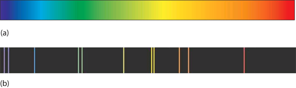
Figure 1 (a) A glowing object gives off a full rainbow of colors, which are noticed only when light is passed through a prism to make a continuous spectrum. (b) However, when electricity is passed through a gas, only certain colors of light are emitted. Here are the colors of light in the line spectrum of Hg.
Why does the light emitted from an electrically excited gas have only certain colors, while light given off by hot objects has a continuous spectrum? For a long time, it was not well explained. Particularly simple was the spectrum of hydrogen gas, which could be described easily by an equation; no other element has a spectrum that is so predictable (Figure 2). Late-nineteenth-century scientists found that the positions of the lines obeyed a pattern given by the equation
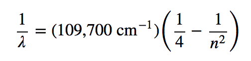
where n = 3, 4, 5, 6,…, but they could not explain why this was so.
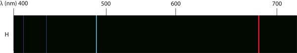
Figure 2 The spectrum of hydrogen was particularly simple and could be predicted by a simple mathematical expression.
In 1913, the Danish scientist Niels Bohr suggested a reason why the hydrogen atom spectrum looked this way. He suggested that the electron in a hydrogen atom could not have any random energy, having only certain fixed values of energy that were indexed by the number n (the same n in the equation above and now called a quantum number. Quantities that have certain specific values are called quantized. Bohr suggested that the energy of the electron in hydrogen was quantized because it was in a specific orbit. Because the energies of the electron can have only certain values, the changes in energies can have only certain values (somewhat similar to a staircase: not only are the stair steps set at specific heights but the height between steps is fixed). Finally, Bohr suggested that the energy of light emitted from electrified hydrogen gas was equal to the energy difference of the electron’s energy states:
[latex]E_{light} =h\nu = \Delta E_{electron}[/latex]
This means that only certain frequencies (and thus, certain wavelengths) of light are emitted. Figure 3 shows a model of the hydrogen atom based on Bohr’s ideas.
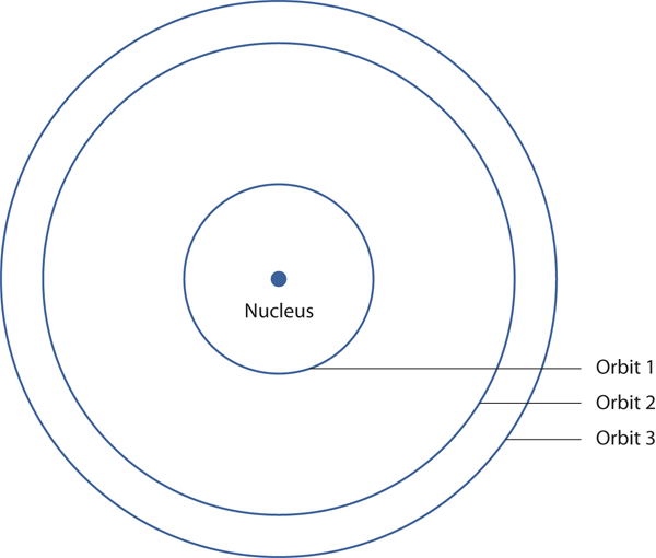
Figure 3 Bohr’s Model. Bohr’s description of the hydrogen atom had specific orbits for the electron, which had quantized energies.
Bohr’s ideas were useful but were applied only to the hydrogen atom. However, later researchers generalized Bohr’s ideas into a new theory called quantum mechanics, which explains the behaviour of electrons as if they were acting as a wave, not as particles. Quantum mechanics predicts two major things: quantized energies for electrons of all atoms (not just hydrogen) and an organization of electrons within atoms. Electrons are no longer thought of as being randomly distributed around a nucleus or restricted to certain orbits (in that regard, Bohr was wrong). Instead, electrons are collected into groups and subgroups that explain much about the chemical behaviour of the atom.
In the quantum-mechanical model of an atom, the state of an electron is described by four quantum numbers, not just the one predicted by Bohr. The first quantum number is called the principle quantum number, represented by n. (n). The principal quantum number largely determines the energy of an electron. Electrons in the same atom that have the same principal quantum number are said to occupy an electron shell of the atom. The principal quantum number can be any nonzero positive integer: 1, 2, 3, 4,….
Within a shell, there may be multiple possible values of the next quantum number, the angular momentum quantum number. Represented by ℓ. (ℓ). The ℓ quantum number has a minor effect on the energy of the electron but also affects the spatial distribution of the electron in three-dimensional space—that is, the shape of an electron’s distribution in space. The value of the ℓ quantum number can be any integer between 0 and n − 1:
ℓ = 0, 1, 2,…, n − 1
Thus, for a given value of n, there are different possible values of ℓ:
| If n equals | ℓ can be |
|---|---|
| 1 | 0 |
| 2 | 0 or 1 |
| 3 | 0, 1, or 2 |
| 4 | 0, 1, 2, or 3 |
and so forth. Electrons within a shell that have the same value of ℓ are said to occupy a subshell in the atom. Commonly, instead of referring to the numerical value of ℓ, a letter represents the value of ℓ (to help distinguish it from the principal quantum number):
| If ℓ equals | The letter is |
|---|---|
| 0 | s |
| 1 | p |
| 2 | d |
| 3 | f |
The next quantum number is called the magnetic quantum number represented by mℓ. (mℓ). For any value of ℓ, there are 2ℓ + 1 possible values of mℓ, ranging from −ℓ to ℓ:
−ℓ ≤ mℓ ≤ ℓ
or
|mℓ| ≤ ℓ
The following explicitly lists the possible values of mℓ for the possible values of ℓ:
| If ℓ equals | The mℓ values can be |
|---|---|
| 0 | 0 |
| 1 | −1, 0, or 1 |
| 2 | −2, −1, 0, 1, or 2 |
| 3 | −3, −2, −1, 0, 1, 2, or 3 |
The particular value of mℓ dictates the orientation of an electron’s distribution in space. When ℓ is zero, mℓ can be only zero, so there is only one possible orientation. When ℓ is 1, there are three possible orientations for an electron’s distribution. When ℓ is 2, there are five possible orientations of electron distribution. This goes on and on for other values of ℓ, but we need not consider any higher values of ℓ here. Each value of mℓ designates a certain orbital. Thus, there is only one orbital when ℓ is zero, three orbitals when ℓ is 1, five orbitals when ℓ is 2, and so forth. The mℓ quantum number has no effect on the energy of an electron unless the electrons are subjected to a magnetic field—hence its name.
The ℓ quantum number dictates the general shape of electron distribution in space (Figure 4). Any s orbital is spherically symmetric (part (a) in Figure 4), and there is only one orbital in any s subshell. Any p orbital has a two-lobed, dumbbell-like shape (part (b) in Figure 4); because there are three of them, we normally represent them as pointing along the x-, y-, and z-axes of Cartesian space. The d orbitals are four-lobed rosettes (part (c) in Figure 4); they are oriented differently in space (the one labelled dz2 has two lobes and a torus instead of four lobes, but it is equivalent to the other orbitals). When there is more than one possible value of mℓ, each orbital is labelled with one of the possible values. It should be noted that the diagrams in Figure 4 are estimates of the electron distribution in space, not surfaces electrons are fixed on.
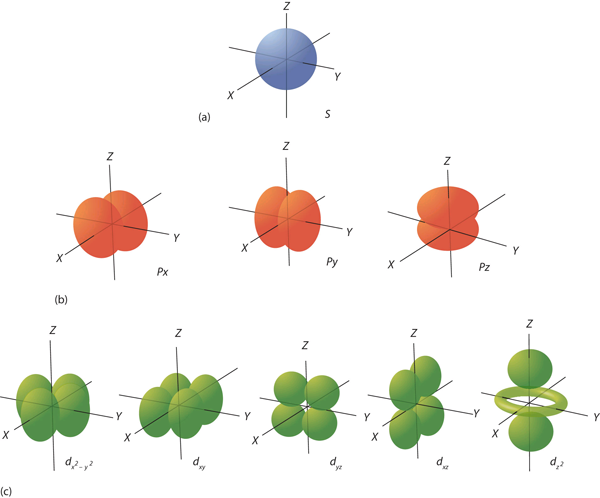
Figure 4 Electron Orbitals. (a) The lone s orbital is spherical in distribution. (b) The three p orbitals are shaped like dumbbells, and each one points in a different direction. (c) The five d orbitals are rosette in shape, except for the dz2 orbital, which is a “dumbbell + torus” combination. They are all oriented in different directions.
The final quantum number is the spin quantum number. Represented by ms. (ms). Electrons and other subatomic particles behave as if they are spinning (we cannot tell if they really are, but they behave as if they are). Electrons themselves have two possible spin states, and because of mathematics, they are assigned the quantum numbers +1/2 and −1/2. These are the only two possible choices for the spin quantum number of an electron.Chemistry Is Everywhere: Neon Lights
A neon light is basically an electrified tube with a small amount of gas in it. Electricity excites electrons in the gas atoms, which then give off light as the electrons go back into a lower energy state. However, many so-called “neon” lights don’t contain neon!
Although we know now that a gas discharge gives off only certain colors of light, without a prism or other component to separate the individual light colors, we see a composite of all the colors emitted. It is not unusual for a certain color to predominate. True neon lights, with neon gas in them, have a reddish-orange light due to the large amount of red-, orange-, and yellow-colored light emitted. However, if you use krypton instead of neon, you get a whitish light, while using argon yields a blue-purple light. A light filled with nitrogen gas glows purple, as does a helium lamp. Other gases—and mixtures of gases—emit other colors of light. Ironically, despite its importance in the development of modern electronic theory, hydrogen lamps emit little visible light and are rarely used for illumination purposes.

Figure 5 The different colors of these “neon” lights are caused by gases other than neon in the discharge tubes. Source: “Neon Internet Cafe open 24 hours” by JustinC is licensed under the Creative Commons Attribution- Share Alike 2.0 Generic license.
The Pauli Exclusion Principle
An electron in an atom is completely described by four quantum numbers: n, l, ml, and ms. The first three quantum numbers define the orbital and the fourth quantum number describes the intrinsic electron property called spin. An Austrian physicist Wolfgang Pauli formulated a general principle that gives the last piece of information that we need to understand the general behavior of electrons in atoms. The Pauli exclusion principle can be formulated as follows: No two electrons in the same atom can have exactly the same set of all the four quantum numbers. What this means is that electrons can share the same orbital (the same set of the quantum numbers n, l, and ml), but only if their spin quantum numbers ms have different values. Since the spin quantum number can only have two values [latex]\left(\pm \frac{1}{2}\right)[/latex], no more than two electrons can occupy the same orbital (and if two electrons are located in the same orbital, they must have opposite spins). Therefore, any atomic orbital can be populated by only zero, one, or two electrons.
Having introduced the basics of atomic structure and quantum mechanics, we can use our understanding of quantum numbers to determine how atomic orbitals relate to one another. This allows us to determine which orbitals are occupied by electrons in each atom. The specific arrangement of electrons in orbitals of an atom determines many of the chemical properties of that atom.
Orbital Energies and Atomic Structure
The energy of atomic orbitals increases as the principal quantum number, n, increases. In any atom with two or more electrons, the repulsion between the electrons makes energies of subshells with different values of l differ so that the energy of the orbitals increases within a shell in the order s < p < d < f. Figure 1 depicts how these two trends in increasing energy relate. The 1s orbital at the bottom of the diagram is the orbital with electrons of lowest energy. The energy increases as we move up to the 2s and then 2p, 3s, and 3p orbitals, showing that the increasing n value has more influence on energy than the increasing l value for small atoms. However, this pattern does not hold for larger atoms. The 3d orbital is higher in energy than the 4s orbital. Such overlaps continue to occur frequently as we move up the chart.
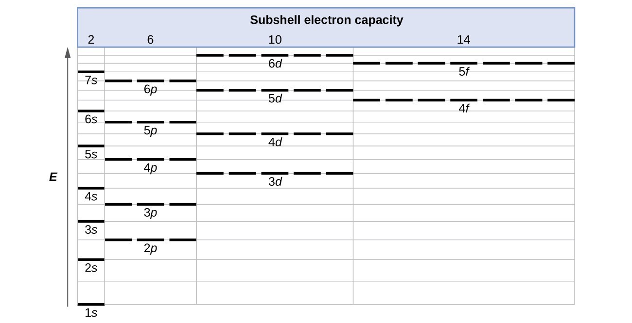
Figure 5. Generalized energy-level diagram for atomic orbitals in an atom with two or more electrons (not to scale).
Electrons in successive atoms on the periodic table tend to fill low-energy orbitals first. Thus, many students find it confusing that, for example, the 5p orbitals fill immediately after the 4d, and immediately before the 6s. The filling order is based on observed experimental results, and has been confirmed by theoretical calculations. As the principal quantum number, n, increases, the size of the orbital increases and the electrons spend more time farther from the nucleus. Thus, the attraction to the nucleus is weaker and the energy associated with the orbital is higher (less stabilized). But this is not the only effect we have to take into account. Within each shell, as the value of l increases, the electrons are less penetrating (meaning there is less electron density found close to the nucleus), in the order s > p > d > f. Electrons that are closer to the nucleus slightly repel electrons that are farther out, offsetting the more dominant electron–nucleus attractions slightly (recall that all electrons have −1 charges, but nuclei have +Z charges). This phenomenon is called shielding and will be discussed in more detail in the next section. Electrons in orbitals that experience more shielding are less stabilized and thus higher in energy. For small orbitals (1s through 3p), the increase in energy due to n is more significant than the increase due to l; however, for larger orbitals the two trends are comparable and cannot be simply predicted. We will discuss methods for remembering the observed order.
The arrangement of electrons in the orbitals of an atom is called the electron configuration of the atom. We describe an electron configuration with a symbol that contains three pieces of information (Figure 6):
- The number of the principal quantum shell, n,
- The letter that designates the orbital type (the subshell, l), and
- A superscript number that designates the number of electrons in that particular subshell.
For example, the notation 2p4 (read “two–p–four”) indicates four electrons in a p subshell (l = 1) with a principal quantum number (n) of 2. The notation 3d8 (read “three–d–eight”) indicates eight electrons in the d subshell (i.e., l = 2) of the principal shell for which n = 3.

Figure 6. The diagram of an electron configuration specifies the subshell (n and l value, with letter symbol) and superscript number of electrons.
The Aufbau Principle
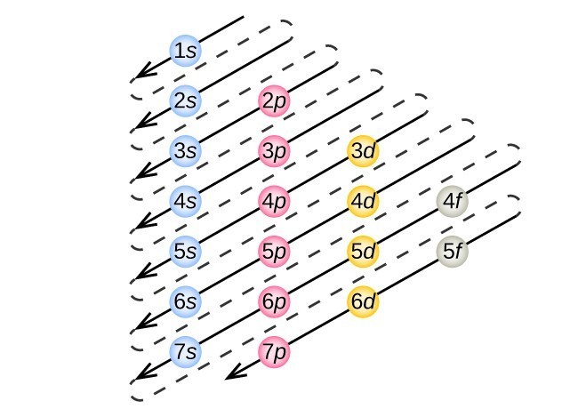
Figure 7. The arrow leads through each subshell in the appropriate filling order for electron configurations. This chart is straightforward to construct. Simply make a column for all the s orbitals with each n shell on a separate row. Repeat for p, d, and f. Be sure to only include orbitals allowed by the quantum numbers (no 1p or 2d, and so forth). Finally, draw diagonal lines from top to bottom as shown.
To determine the electron configuration for any particular atom, we can “build” the structures in the order of atomic numbers. Beginning with hydrogen, and continuing across the periods of the periodic table, we add one proton at a time to the nucleus and one electron to the proper subshell until we have described the electron configurations of all the elements.
This procedure is called the Aufbau principle, from the German word Aufbau (“to build up”). Each added electron occupies the subshell of lowest energy available (in the order shown in Figure 7), subject to the limitations imposed by the allowed quantum numbers according to the Pauli exclusion principle. Electrons enter higher-energy subshells only after lower-energy subshells have been filled to capacity. Figure 7 illustrates the traditional way to remember the filling order for atomic orbitals.
Writing Electron Configurations
Chemists use an electron configuration, to represent the organization of electrons in shells and subshells in an atom. An electron configuration simply lists the shell and subshell labels, with a right superscript giving the number of electrons in that subshell. The shells and subshells are listed in the order of filling.
For example, an H atom has a single electron in the 1s subshell. Its electron configuration is
[latex]H: 1s^{1}[/latex]
He has two electrons in the 1s subshell. Its electron configuration is
[latex]He: 1s^{2}[/latex]
The three electrons for Li are arranged in the 1s subshell (two electrons) and the 2s subshell (one electron). The electron configuration of Li is
[latex]Li: 1s^{2}2s^{1}[/latex]
Be has four electrons, two in the 1s subshell and two in the 2s subshell. Its electron configuration is
[latex]Be: 1s^{2}2s^{2}[/latex]
Now that the 2s subshell is filled, electrons in larger atoms must go into the 2p subshell, which can hold a maximum of six electrons. The next six elements progressively fill up the 2p subshell:
[latex]B: 1s^{2}2s^{2}2p^{1}[/latex]
[latex]C: 1s^{2}2s^{2}2p^{2}[/latex]
[latex]N: 1s^{2}2s^{2}2p^{3}[/latex]
[latex]O: 1s^{2}2s^{2}2p^{4}[/latex]
[latex]F: 1s^{2}2s^{2}2p^{5}[/latex]
[latex]Ne: 1s^{2}2s^{2}2p^{6}[/latex]
Now that the 2p subshell is filled (all possible subshells in the n = 2 shell), the next electron for the next-larger atom must go into the n = 3 shell, s subshell.
Example 1: Electron Configuration
What is the electron configuration for Na, which has 11 electrons?
Check Your Learning
What is the electron configuration for Mg, which has 12 electrons?
Example 2: Electron Configuration
What is the predicted electron configuration for Sn, which has 50 electrons?
Check Your Learning
What is the electron configuration for Ba, which has 56 electrons?
Abbreviated Electron Configurations
As the previous example demonstrated, electron configurations can get fairly long. An abbreviated electron configuration, also known as a noble gas abbreviated electron configuration, uses one of the elements from the last column of the periodic table, which contains what are called the noble gases, to represent the core of electrons up to that element. Then the remaining electrons are listed explicitly. For example, the abbreviated electron configuration for Li, which has three electrons, would be
Li: [He]2s1
where [He] represents the two-electron core that is equivalent to He’s electron configuration. The square brackets represent the electron configuration of a noble gas. This is not much of an abbreviation. However, consider the abbreviated electron configuration for W, which has 74 electrons:
W: [Xe]6s24f145d4
This is a significant simplification over an explicit listing of all 74 electrons. So for larger elements, the abbreviated electron configuration can be a very useful shorthand.
Example 7: Abbreviated Electron Configuration
What is the abbreviated electron configuration for P, which has 15 electrons?
Check Your Learning
What is the abbreviated electron configuration for Rb, which has 37 electrons?
There are some exceptions to the rigorous filling of subshells by electrons. In many cases, an electron goes from a higher-numbered shell to a lower-numbered but later-filled subshell to fill the later-filled subshell. One example is Ag. With 47 electrons, its electron configuration is predicted to be
Ag: [Kr]5s24d9
However, experiments have shown that the electron configuration is actually
Ag: [Kr]5s14d10
This, then, qualifies as an exception to our expectations. At this point, you do not need to worry about the exceptions; we will ignore these exceptions in this course.
Electron Configuration Energy Diagrams
We have just seen that electrons fill orbitals in shells and subshells in a regular pattern, but why does it follow this pattern? There are three principles which should be followed to properly fill electron orbital energy diagrams:
- The Aufbau principle
- The Pauli exclusion principle
- Hund’s rule
The overall pattern of the electron shell filling order emerges from the Aufbau principle (German for “building up”): electrons fill the lowest energy orbitals first. Increasing the principle quantum number, n, increases orbital energy levels, as the electron density becomes more spread out away from the nucleus. In many-electron atoms (all atoms except hydrogen), the energy levels of subshells varies due to electron-electron repulsions. The trend that emerges is that energy levels increase with value of the angular momentum quantum number, l, for orbitals sharing the same principle quantum number, n. This is demonstrated in Figure 7, where each line represents an orbital, and each set of lines at the same energy represents a subshell of orbitals.
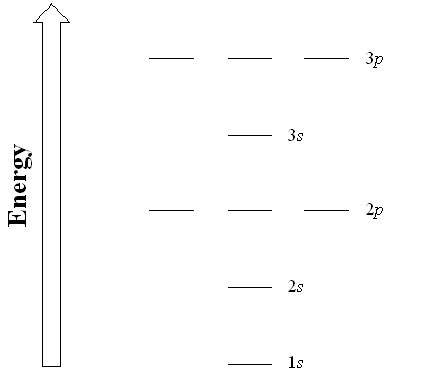
Figure 7. Generic energy diagram of orbitals in a multi-electron atom.
As previously discussed, the Pauli exclusion principle states that we can only fill each orbital with a maximum of two electrons of opposite spin. But how should we fill multiple orbitals of the same energy level within a subshell (eg. The three orbitals in the 2p subshell)? Orbitals of the same energy level are known as degenerate orbitals, and we fill them using Hund’s rule: place one electron into each degenerate orbital first, before pairing them in the same orbital.
Let’s examine a few examples to demonstrate the use of the three principles.
Boron is atomic number 5, and therefore has 5 electrons. First fill the lowest energy 1s orbital with two electrons of opposite spin, then the 2s orbital with 2 electrons of opposite spin and finally place the last electron into any of the three degenerate 2p orbitals (Figure 8).
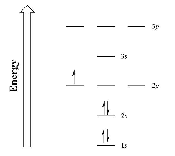
Figure 8. Boron electron configuration energy diagram
Moving across the periodic table, we follow Hund’s rule and add an additional electron to each degenerate 2p orbital for each subsequent element (Figure 9). At oxygen we can finally pair up and fill one of the degenerate 2p orbitals.
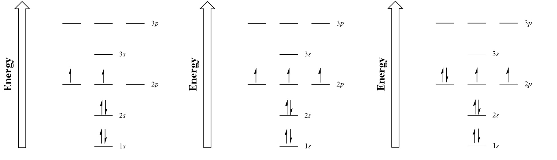
Figure 9. Electron configuration energy diagrams for carbon, nitrogen and oxygen.
Key Takeaways
- The Pauli exclusion principle limits the number of electrons in the subshells and shells.
- Electrons in larger atoms fill shells and subshells in a regular pattern that we can follow.
- Electron configurations are a shorthand method of indicating what subshells electrons occupy in atoms.
- Abbreviated electron configurations are a simpler way of representing electron configurations for larger atoms.
- Exceptions to the strict filling of subshells with electrons occur.
- Electron configurations are assigned from lowest to highest energy following the Aufbau principle
- One electron is placed in each degenerate orbital before pairing electrons following Hund’s rule.
- Electron configuration energy diagrams follow three principles: the Aufbau principle, the Pauli exclusion principle and Hund’s rule.
Exercises
1. How many subshells are completely filled with electrons for Na? How many subshells are unfilled?
2. How many subshells are completely filled with electrons for Mg? How many subshells are unfilled?
3. What is the maximum number of electrons in the entire n = 2 shell?
4. What is the maximum number of electrons in the entire n = 4 shell?
5. Write the complete electron configuration for each atom.
a) Si, 14 electrons
b) Sc, 21 electrons
6. Write the complete electron configuration for each atom.
a) Br, 35 electrons
b) Be, 4 electrons
7. Write the complete electron configuration for each atom.
a) Cd, 48 electrons
b) Mg, 12 electrons
8. Write the complete electron configuration for each atom.
a) Cs, 55 electrons
b) Ar, 18 electrons
9. Write the abbreviated electron configuration for each atom in Exercise 7.
10. Write the abbreviated electron configuration for each atom in Exercise 8.
11. Write the abbreviated electron configuration for each atom in Exercise 9.
12. Write the abbreviated electron configuration for each atom in Exercise 10.
13. Draw electron configuration energy diagrams for potassium, and bromine.


Glossary
Aufbau principle: procedure in which the electron configuration of the elements is determined by “building” them in order of atomic numbers, adding one proton to the nucleus and one electron to the proper subshell at a time
core electron: electron in an atom that occupies the orbitals of the inner shells
electron configuration: electronic structure of an atom in its ground state given as a listing of the orbitals occupied by the electrons
Hund’s rule: every orbital in a subshell is singly occupied with one electron before any one orbital is doubly occupied, and all electrons in singly occupied orbitals have the same spin
orbital diagram: pictorial representation of the electron configuration showing each orbital as a box and each electron as an arrow
valence electrons: electrons in the outermost or valence shell (highest value of n) of a ground-state atom; determine how an element reacts
valence shell: outermost shell of electrons in a ground-state atom; for main group elements, the orbitals with the highest n level (s and p subshells) are in the valence shell, while for transition metals, the highest energy s and d subshells make up the valence shell and for inner transition elements, the highest s, d, and f subshells are included
Candela Citations
- Introductory Chemistry- 1st Canadian Edition . Authored by: Jessie A. Key and David W. Ball. Provided by: BCCampus. Located at: https://opentextbc.ca/introductorychemistry/. License: CC BY-NC-SA: Attribution-NonCommercial-ShareAlike. License Terms: Download this book for free at http://open.bccampus.ca
- Chemistry. Provided by: OpenStax College. Located at: http://openstaxcollege.org. License: CC BY: Attribution. License Terms: Download for free at https://openstaxcollege.org/textbooks/chemistry/get