It frequently happens that a dependent variable (y) in which we are interested is related to more than one independent variable. If this relationship can be estimated, it may enable us to make more precise predictions of the dependent variable than would be possible by a simple linear regression. Regressions based on more than one independent variable are called multiple regressions.
Multiple linear regression is an extension of simple linear regression and many of the ideas we examined in simple linear regression carry over to the multiple regression setting. For example, scatterplots, correlation, and least squares method are still essential components for a multiple regression.
For example, a habitat suitability index (used to evaluate the impact on wildlife habitat from land use changes) for ruffed grouse might be related to three factors:
x1 = stem density
x2 = percent of conifers
x3 = amount of understory herbaceous matter
A researcher would collect data on these variables and use the sample data to construct a regression equation relating these three variables to the response. The researcher will have questions about his model similar to a simple linear regression model.
- How strong is the relationship between y and the three predictor variables?
- How well does the model fit?
- Have any important assumptions been violated?
- How good are the estimates and predictions?
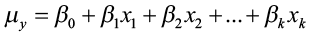
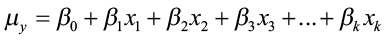
The general linear regression model takes the form of
 ,
,
with the mean value of y given as
 ,
,
where:
- y is the random response variable and μy is the mean value of y,
- β0, β1, β2, and βk are the parameters to be estimated based on the sample data,
- x1, x2,…, xk are the predictor variables that are assumed to be non-random or fixed and measured without error, and k is the number of predictor variable,
- and ε is the random error, which allows each response to deviate from the average value of y. The errors are assumed to be independent, have a mean of zero and a common variance (σ2), and are normally distributed.
As you can see, the multiple regression model and assumptions are very similar to those for a simple linear regression model with one predictor variable. Examining residual plots and normal probability plots for the residuals is key to verifying the assumptions.
Correlation
As with simple linear regression, we should always begin with a scatterplot of the response variable versus each predictor variable. Linear correlation coefficients for each pair should also be computed. Instead of computing the correlation of each pair individually, we can create a correlation matrix, which shows the linear correlation between each pair of variables under consideration in a multiple linear regression model.
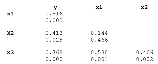
Table 1. A correlation matrix.
In this matrix, the upper value is the linear correlation coefficient and the lower value is the p-value for testing the null hypothesis that a correlation coefficient is equal to zero. This matrix allows us to see the strength and direction of the linear relationship between each predictor variable and the response variable, but also the relationship between the predictor variables. For example, y and x1 have a strong, positive linear relationship with r = 0.816, which is statistically significant because p = 0.000. We can also see that predictor variables x1 and x3 have a moderately strong positive linear relationship (r = 0.588) that is significant (p = 0.001).
There are many different reasons for selecting which explanatory variables to include in our model (see Model Development and Selection), however, we frequently choose the ones that have a high linear correlation with the response variable, but we must be careful. We do not want to include explanatory variables that are highly correlated among themselves. We need to be aware of any multicollinearity between predictor variables.
Multicollinearity exists between two explanatory variables if they have a strong linear relationship.
For example, if we are trying to predict a person’s blood pressure, one predictor variable would be weight and another predictor variable would be diet. Both predictor variables are highly correlated with blood pressure (as weight increases blood pressure typically increases, and as diet increases blood pressure also increases). But, both predictor variables are also highly correlated with each other. Both of these predictor variables are conveying essentially the same information when it comes to explaining blood pressure. Including both in the model may lead to problems when estimating the coefficients, as multicollinearity increases the standard errors of the coefficients. This means that coefficients for some variables may be found not to be significantly different from zero, whereas without multicollinearity and with lower standard errors, the same coefficients might have been found significant. Ways to test for multicollinearity are not covered in this text, however a general rule of thumb is to be wary of a linear correlation of less than -0.7 and greater than 0.7 between two predictor variables. Always examine the correlation matrix for relationships between predictor variables to avoid multicollinearity issues.
Estimation
Estimation and inference procedures are also very similar to simple linear regression. Just as we used our sample data to estimate β0 and β1 for our simple linear regression model, we are going to extend this process to estimate all the coefficients for our multiple regression models.
With the simpler population model
 x
x
β1 is the slope and tells the user what the change in the response would be as the predictor variable changes. With multiple predictor variables, and therefore multiple parameters to estimate, the coefficients β1, β2, β3 and so on are called partial slopes or partial regression coefficients. The partial slope βi measures the change in y for a one-unit change in xi when all other independent variables are held constant. These regression coefficients must be estimated from the sample data in order to obtain the general form of the estimated multiple regression equation
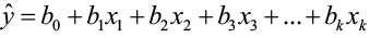
and the population model
where k = the number of independent variables (also called predictor variables)
ŷ = the predicted value of the dependent variable (computed by using the multiple regression equation)
x1, x2, …, xk = the independent variables
β0 is the y-intercept (the value of y when all the predictor variables equal 0)
b0 is the estimate of β0 based on that sample data
β1, β2, β3,…βk are the coefficients of the independent variables x1, x2, …, xk
b1, b2, b3, …, bk are the sample estimates of the coefficients β1, β2, β3,…βk
The method of least-squares is still used to fit the model to the data. Remember that this method minimizes the sum of the squared deviations of the observed and predicted values (SSE).
The analysis of variance table for multiple regression has a similar appearance to that of a simple linear regression.
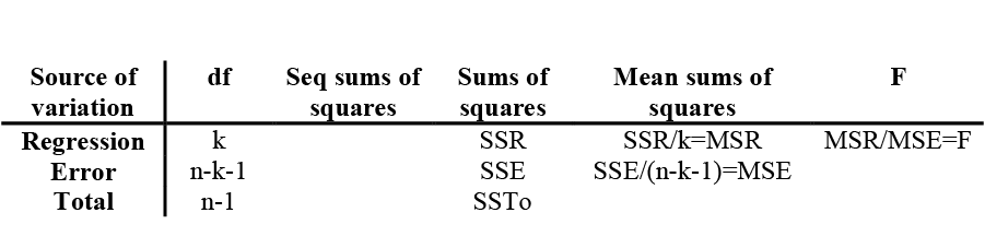
Table 2. ANOVA table.
Where k is the number of predictor variables and n is the number of observations.
The best estimate of the random variation σ2—the variation that is unexplained by the predictor variables—is still s2, the MSE. The regression standard error, s, is the square root of the MSE.
A new column in the ANOVA table for multiple linear regression shows a decomposition of SSR, in which the conditional contribution of each predictor variable given the variables already entered into the model is shown for the order of entry that you specify in your regression. These conditional or sequential sums of squares each account for 1 regression degree of freedom, and allow the user to see the contribution of each predictor variable to the total variation explained by the regression model by using the ratio:

Adjusted R2
In simple linear regression, we used the relationship between the explained and total variation as a measure of model fit:
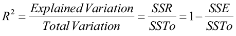
Notice from this definition that the value of the coefficient of determination can never decrease with the addition of more variables into the regression model. Hence, R2 can be artificially inflated as more variables (significant or not) are included in the model. An alternative measure of strength of the regression model is adjusted for degrees of freedom by using mean squares rather than sums of squares:
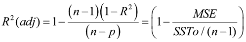
The adjusted R2 value represents the percentage of variation in the response variable explained by the independent variables, corrected for degrees of freedom. Unlike R2, the adjusted R2 will not tend to increase as variables are added and it will tend to stabilize around some upper limit as variables are added.
Tests of Significance
Recall in the previous chapter we tested to see if y and x were linearly related by testing
|
H0: β1 = 0 |
H1: β1 ≠ 0 |
with the t-test (or the equivalent F-test). In multiple linear regression, there are several partial slopes and the t-test and F-test are no longer equivalent. Our question changes: Is the regression equation that uses information provided by the predictor variables x1, x2, x3, …, xk, better than the simple predictor  (the mean response value), which does not rely on any of these independent variables?
H0: β1 = β2 = β3 = …=βk = 0
H1: At least one of β1, β2 , β3 , …βk ≠ 0
The F-test statistic is used to answer this question and is found in the ANOVA table.

This test statistic follows the F-distribution with df1 = k and df2 = (n-k-1). Since the exact p-value is given in the output, you can use the Decision Rule to answer the question.
If the p-value is less than the level of significance, reject the null hypothesis.
Rejecting the null hypothesis supports the claim that at least one of the predictor variables has a significant linear relationship with the response variable. The next step is to determine which predictor variables add important information for prediction in the presence of other predictors already in the model. To test the significance of the partial regression coefficients, you need to examine each relationship separately using individual t-tests.
|
H0: βi = 0 |
H1: βi ≠ 0 |
 with df = (n-k-1)
where SE(bi) is the standard error of bi. Exact p-values are also given for these tests. Examining specific p-values for each predictor variable will allow you to decide which variables are significantly related to the response variable. Typically, any insignificant variables are removed from the model, but remember these tests are done with other variables in the model. A good procedure is to remove the least significant variable and then refit the model with the reduced data set. With each new model, always check the regression standard error (lower is better), the adjusted R2 (higher is better), the p-values for all predictor variables, and the residual and normal probability plots.
Because of the complexity of the calculations, we will rely on software to fit the model and give us the regression coefficients. Don’t forget… you always begin with scatterplots. Strong relationships between predictor and response variables make for a good model.
Example 1
A researcher collected data in a project to predict the annual growth per acre of upland boreal forests in southern Canada. They hypothesized that cubic foot volume growth (y) is a function of stand basal area per acre (x1), the percentage of that basal area in black spruce (x2), and the stand’s site index for black spruce (x3). α = 0.05.
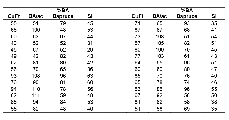
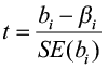
Table 3. Observed data for cubic feet, stand basal area, percent basal area in black spruce, and site index.
Scatterplots of the response variable versus each predictor variable were created along with a correlation matrix.
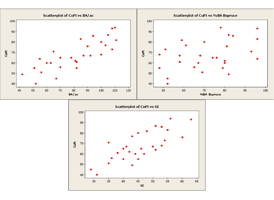
Figure 1. Scatterplots of cubic feet versus basal area, percent basal area in black spruce, and site index.
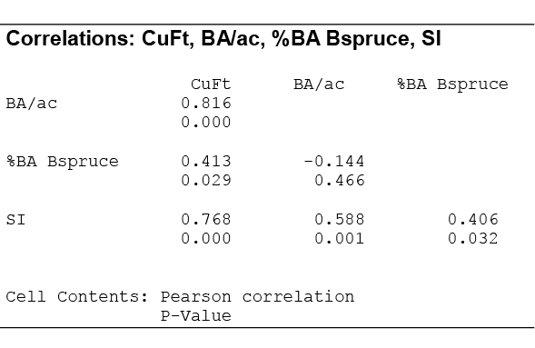
Table 4. Correlation matrix.
As you can see from the scatterplots and the correlation matrix, BA/ac has the strongest linear relationship with CuFt volume (r = 0.816) and %BA in black spruce has the weakest linear relationship (r = 0.413). Also of note is the moderately strong correlation between the two predictor variables, BA/ac and SI (r = 0.588). All three predictor variables have significant linear relationships with the response variable (volume) so we will begin by using all variables in our multiple linear regression model. The Minitab output is given below.
We begin by testing the following null and alternative hypotheses:
H0: β1 = β2 = β3 = 0
H1: At least one of β1, β2 , β3 ≠ 0
General Regression Analysis: CuFt versus BA/ac, SI, %BA Bspruce
|
Regression Equation |
||||||
|
CuFt = -19.3858 + 0.591004 BA/ac + 0.0899883 SI + 0.489441 %BA Bspruce |
||||||
|
Coefficients |
||||||
|
Term |
Coef |
SE Coef |
T |
P |
95% CI |
|
|
Constant |
-19.3858 |
4.15332 |
-4.6675 |
0.000 |
(-27.9578, -10.8137) |
|
|
BA/ac |
0.5910 |
0.04294 |
13.7647 |
0.000 |
(0.5024, 0.6796) |
|
|
SI |
0.0900 |
0.11262 |
0.7991 |
0.432 |
(-0.1424, 0.3224) |
|
|
%BA Bspruce |
0.4894 |
0.05245 |
9.3311 |
0.000 |
(0.3812, 0.5977) |
|
|
Summary of Model |
||||||
|
S = 3.17736 |
R-Sq = 95.53% |
R-Sq(adj) = 94.97% |
||||
|
PRESS = 322.279 |
R-Sq(pred) = 94.05% |
|||||
|
Analysis of Variance |
||||||
|
Source |
DF |
Seq SS |
Adj SS |
Adj MS |
F |
P |
|
Regression |
3 |
5176.56 |
5176.56 |
1725.52 |
170.918 |
0.000000 |
|
BA/ac |
1 |
3611.17 |
1912.79 |
1912.79 |
189.467 |
0.000000 |
|
SI |
1 |
686.37 |
6.45 |
6.45 |
0.638 |
0.432094 |
|
%BA Bspruce |
1 |
879.02 |
879.02 |
879.02 |
87.069 |
0.000000 |
|
Error |
24 |
242.30 |
242.30 |
10.10 |
||
|
Total |
27 |
5418.86 |
||||
The F-test statistic (and associated p-value) is used to answer this question and is found in the ANOVA table. For this example, F = 170.918 with a p-value of 0.00000. The p-value is smaller than our level of significance (0.0000<0.05) so we will reject the null hypothesis. At least one of the predictor variables significantly contributes to the prediction of volume.
The coefficients for the three predictor variables are all positive indicating that as they increase cubic foot volume will also increase. For example, if we hold values of SI and %BA Bspruce constant, this equation tells us that as basal area increases by 1 sq. ft., volume will increase an additional 0.591004 cu. ft. The signs of these coefficients are logical, and what we would expect. The adjusted R2 is also very high at 94.97%.
The next step is to examine the individual t-tests for each predictor variable. The test statistics and associated p-values are found in the Minitab output and repeated below:
|
Coefficients |
|||||
|
Term |
Coef |
SE Coef |
T |
P |
95% CI |
|
Constant |
-19.3858 |
4.15332 |
-4.6675 |
0.000 |
(-27.9578, -10.8137) |
|
BA/ac |
0.5910 |
0.04294 |
13.7647 |
0.000 |
( 0.5024, 0.6796) |
|
SI |
0.0900 |
0.11262 |
0.7991 |
0.432 |
( -0.1424, 0.3224) |
|
%BA Bspruce |
0.4894 |
0.05245 |
9.3311 |
0.000 |
( 0.3812, 0.5977) |
The predictor variables BA/ac and %BA Bspruce have t-statistics of 13.7647 and 9.3311 and p-values of 0.0000, indicating that both are significantly contributing to the prediction of volume. However, SI has a t-statistic of 0.7991 with a p-value of 0.432. This variable does not significantly contribute to the prediction of cubic foot volume.
This result may surprise you as SI had the second strongest relationship with volume, but don’t forget about the correlation between SI and BA/ac (r = 0.588). The predictor variable BA/ac had the strongest linear relationship with volume, and using the sequential sums of squares, we can see that BA/ac is already accounting for 70% of the variation in cubic foot volume (3611.17/5176.56 = 0.6976). The information from SI may be too similar to the information in BA/ac, and SI only explains about 13% of the variation on volume (686.37/5176.56 = 0.1326) given that BA/ac is already in the model.
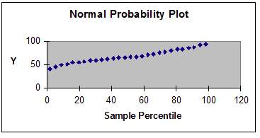
The next step is to examine the residual and normal probability plots. A single outlier is evident in the otherwise acceptable plots.
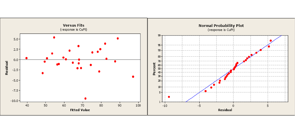
Figure 2. Residual and normal probability plots.
So where do we go from here?
We will remove the non-significant variable and re-fit the model excluding the data for SI in our model. The Minitab output is given below.
General Regression Analysis: CuFt versus BA/ac, %BA Bspruce
|
Regression Equation |
||||||
|
CuFt = -19.1142 + 0.615531 BA/ac + 0.515122 %BA Bspruce |
||||||
|
Coefficients |
||||||
|
Term |
Coef |
SE Coef |
T |
P |
95% CI |
|
|
Constant |
-19.1142 |
4.10936 |
-4.6514 |
0.000 |
(-27.5776, -10.6508) |
|
|
BA/ac |
0.6155 |
0.02980 |
20.6523 |
0.000 |
(0.5541, 0.6769) |
|
|
%BA Bspruce |
0.5151 |
0.04115 |
12.5173 |
0.000 |
(0.4304, 0.5999) |
|
|
Summary of Model |
||||||
|
S = 3.15431 |
R-Sq = 95.41% |
R-Sq(adj) = 95.04% |
||||
|
PRESS = 298.712 |
R-Sq(pred) = 94.49% |
|||||
|
Analysis of Variance |
||||||
|
Source |
DF |
SeqSS |
AdjSS |
AdjMS |
F |
P |
|
Regression |
2 |
5170.12 |
5170.12 |
2585.06 |
259.814 |
0.0000000 |
|
BA/ac |
1 |
3611.17 |
4243.71 |
4243.71 |
426.519 |
0.0000000 |
|
%BA Bspruce |
1 |
1558.95 |
1558.95 |
1558.95 |
156.684 |
0.0000000 |
|
Error |
25 |
248.74 |
248.74 |
9.95 |
||
|
Total |
27 |
5418.86 |
||||
We will repeat the steps followed with our first model. We begin by again testing the following hypotheses:
H0: β1 = β2 = β3 = 0
H1: At least one of β1, β2 , β3 ≠ 0
This reduced model has an F-statistic equal to 259.814 and a p-value of 0.0000. We will reject the null hypothesis. At least one of the predictor variables significantly contributes to the prediction of volume. The coefficients are still positive (as we expected) but the values have changed to account for the different model.
The individual t-tests for each coefficient (repeated below) show that both predictor variables are significantly different from zero and contribute to the prediction of volume.
|
Coefficients |
|||||
|
Term |
Coef |
SE Coef |
T |
P |
95% CI |
|
Constant |
-19.1142 |
4.10936 |
-4.6514 |
0.000 |
(-27.5776, -10.6508) |
|
BA/ac |
0.6155 |
0.02980 |
20.6523 |
0.000 |
( 0.5541, 0.6769) |
|
%BA Bspruce |
0.5151 |
0.04115 |
12.5173 |
0.000 |
( 0.4304, 0.5999) |
Notice that the adjusted R2 has increased from 94.97% to 95.04% indicating a slightly better fit to the data. The regression standard error has also changed for the better, decreasing from 3.17736 to 3.15431 indicating slightly less variation of the observed data to the model.
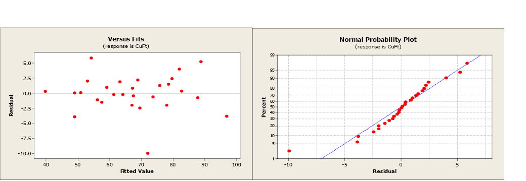
Figure 3. Residual and normal probability plots.
The residual and normal probability plots have changed little, still not indicating any issues with the regression assumption. By removing the non-significant variable, the model has improved.
Model Development and Selection
There are many different reasons for creating a multiple linear regression model and its purpose directly influences how the model is created. Listed below are several of the more commons uses for a regression model:
- Describing the behavior of your response variable
- Predicting a response or estimating the average response
- Estimating the parameters (β0, β1, β2, …)
- Developing an accurate model of the process
Depending on your objective for creating a regression model, your methodology may vary when it comes to variable selection, retention, and elimination.
When the object is simple description of your response variable, you are typically less concerned about eliminating non-significant variables. The best representation of the response variable, in terms of minimal residual sums of squares, is the full model, which includes all predictor variables available from the data set. It is less important that the variables are causally related or that the model is realistic.
A common reason for creating a regression model is for prediction and estimating. A researcher wants to be able to define events within the x-space of data that were collected for this model, and it is assumed that the system will continue to function as it did when the data were collected. Any measurable predictor variables that contain information on the response variable should be included. For this reason, non-significant variables may be retained in the model. However, regression equations with fewer variables are easier to use and have an economic advantage in terms of data collection. Additionally, there is a greater confidence attached to models that contain only significant variables.
If the objective is to estimate the model parameters, you will be more cautious when considering variable elimination. You want to avoid introducing a bias by removing a variable that has predictive information about the response. However, there is a statistical advantage in terms of reduced variance of the parameter estimates if variables truly unrelated to the response variable are removed.
Building a realistic model of the process you are studying is often a primary goal of much research. It is important to identify the variables that are linked to the response through some causal relationship. While you can identify which variables have a strong correlation with the response, this only serves as an indicator of which variables require further study. The principal objective is to develop a model whose functional form realistically reflects the behavior of a system.
The following figure is a strategy for building a regression model.
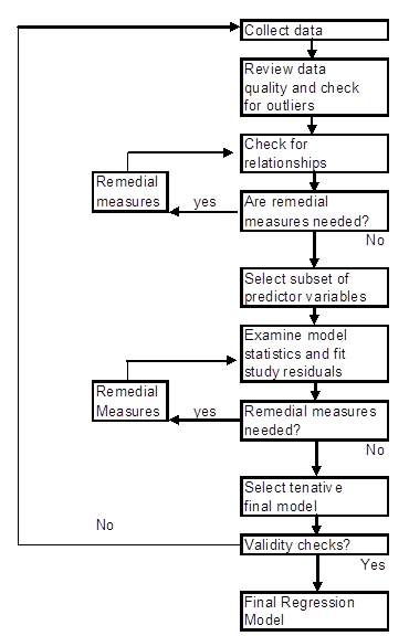
Figure 4. Strategy for building a regression model.
Software Solutions
Minitab
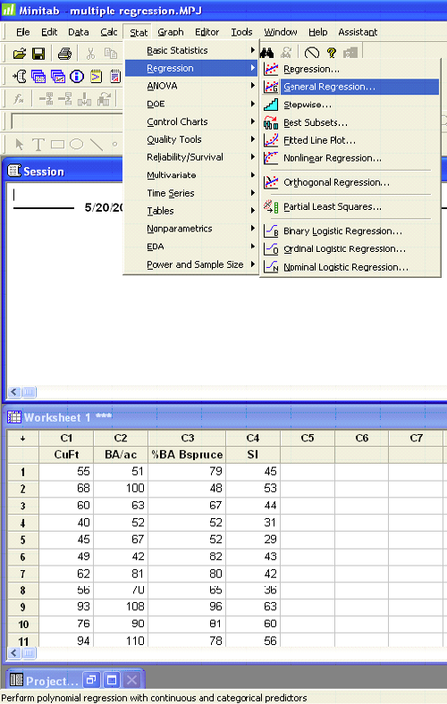
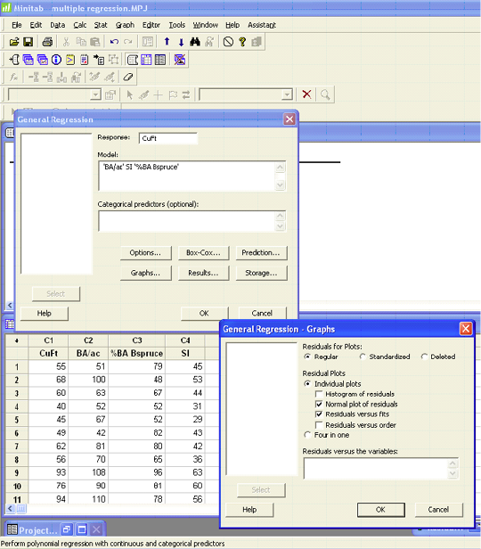
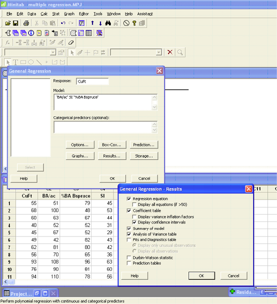
The output and plots are given in the previous example.
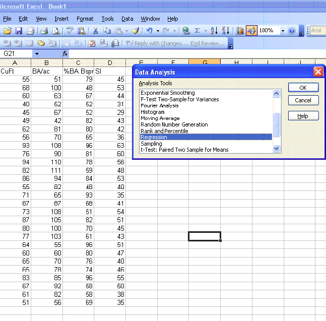
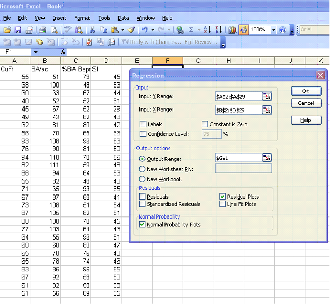
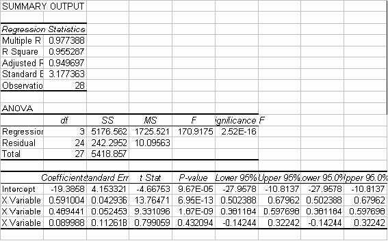
Excel
Candela Citations
- Natural Resources Biometrics. Authored by: Diane Kiernan. Located at: https://textbooks.opensuny.org/natural-resources-biometrics/. Project: Open SUNY Textbooks. License: CC BY-NC-SA: Attribution-NonCommercial-ShareAlike