In mainstream economics, economic surplus, also known as total welfare or Marshallian surplus (after Alfred Marshall), refers to two related quantities. Consumer surplus or consumers’ surplus is the monetary gain obtained by consumers because they are able to purchase a product for a price that is less than the highest price that they would be willing to pay. Producer surplus or producers’ surplus is the amount that producers benefit by selling at a market price that is higher than the least that they would be willing to sell for; this is roughly equal to profit (since producers are not normally willing to sell at a loss, and are normally indifferent to selling at a breakeven price)
On a standard supply and demand diagram, consumer surplus is the area (triangular if the supply and demand curves are linear) above the equilibrium price of the good and below the demand curve. This reflects the fact that consumers would have been willing to buy a single unit of the good at a price higher than the equilibrium price, a second unit at a price below that but still above the equilibrium price, etc., yet they in fact pay just the equilibrium price for each unit they buy.
Likewise, in the supply-demand diagram, producer surplus is the area below the equilibrium price but above the supply curve. This reflects the fact that producers would have been willing to supply the first unit at a price lower than the equilibrium price, the second unit at a price above that but still below the equilibrium price, etc., yet they in fact receive the equilibrium price for all the units they sell.
Consumer surplus
Consumer surplus is the difference between the maximum price a consumer is willing to pay and the actual price they do pay. If a consumer is willing to pay more for a unit of a good than the current asking price, they are getting more benefit from the purchased product than they would if the price was their maximum willingness to pay. They are receiving the same benefit, the obtainment of the good, with a smaller cost as they are spending less than they would if they were charged their maximum willingness to pay.[3] An example of a good with generally high consumer surplus is drinking water. People would pay very high prices for drinking water, as they need it to survive. The difference in the price that they would pay, if they had to, and the amount that they pay now is their consumer surplus. The utility of the first few litres of drinking water is very high (as it prevents death), so the first few litres would likely have more consumer surplus than subsequent litres.
The maximum amount a consumer would be willing to pay for a given quantity of a good is the sum of the maximum price they would pay for the first unit, the (lower) maximum price they would be willing to pay for the second unit, etc. Typically these prices are decreasing; they are given by the individual demand curve, which must be generated by a rational consumer who maximizes utility subject to a budget constraint. Because the demand curve is downward sloping, there is diminishing marginal utility. Diminishing marginal utility means a person receives less additional utility from an additional unit. However, the price of a product is constant for every unit at the equilibrium price. The extra money someone would be willing to pay for the number units of a product less than the equilibrium quantity and at a higher price than the equilibrium price for each of these quantities is the benefit they receive from purchasing these quantities. For a given price the consumer buys the amount for which the consumer surplus is highest. The consumer’s surplus is highest at the largest number of units for which, even for the last unit, the maximum willingness to pay is not below the market price.
Consumer surplus can be used as a measurement of social welfare, first shown by Willig (1976). For a single price change, consumer surplus can provide an approximation of changes in welfare. With multiple price and/or income changes, however, consumer surplus cannot be used to approximate economic welfare because it is not single-valued anymore. More modern methods are developed later to estimate the welfare effect of price changes using consumer surplus.
The aggregate consumers’ surplus is the sum of the consumer’s surplus for all individual consumers. This can be represented graphically as shown in the above graph of the market demand and supply curves. It can also be said to be the maxim of satisfaction a consumer derives from particular goods and services.
Consider a market for tablet computers, as shown in Figure 1. The equilibrium price is $80 and the equilibrium quantity is 28 million. To see the benefits to consumers, look at the segment of the demand curve above the equilibrium point and to the left. This portion of the demand curve shows that at least some demanders would have been willing to pay more than $80 for a tablet.
For example, point J shows that if the price was $90, 20 million tablets would be sold. Those consumers who would have been willing to pay $90 for a tablet based on the utility they expect to receive from it, but who were able to pay the equilibrium price of $80, clearly received a benefit beyond what they had to pay for. Remember, the demand curve traces consumers’ willingness to pay for different quantities. The amount that individuals would have been willing to pay, minus the amount that they actually paid, is called consumer surplus. Consumer surplus is the area labeled F—that is, the area above the market price and below the demand curve.
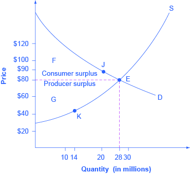
The supply curve shows the quantity that firms are willing to supply at each price. For example, point K in Figure 1 illustrates that, at $45, firms would still have been willing to supply a quantity of 14 million. Those producers who would have been willing to supply the tablets at $45, but who were instead able to charge the equilibrium price of $80, clearly received an extra benefit beyond what they required to supply the product. The amount that a seller is paid for a good minus the seller’s actual cost is called producer surplus. In Figure 1, producer surplus is the area labeled G—that is, the area between the market price and the segment of the supply curve below the equilibrium.
The sum of consumer surplus and producer surplus is social surplus, also referred to as economic surplus or total surplus. In Figure 1, social surplus would be shown as the area F + G. Social surplus is larger at equilibrium quantity and price than it would be at any other quantity. This demonstrates the economic efficiency of the market equilibrium. In addition, at the efficient level of output, it is impossible to produce greater consumer surplus without reducing producer surplus, and it is impossible to produce greater producer surplus without reducing consumer surplus.
Candela Citations
- Provided by: Wikipedia. Located at: https://en.wikipedia.org/wiki/Economic_surplus. License: CC BY-SA: Attribution-ShareAlike
- Located at: https://opentextbc.ca/principlesofeconomics/chapter/3-5-demand-supply-and-efficiency/. Project: Principles of Economics. License: CC BY: Attribution
- Authored by: Jason Welker. Located at: https://www.youtube.com/watch?v=PXzfJtCr9bA&feature=emb_logo. License: All Rights Reserved
- Authored by: Jason Welker. Located at: https://www.youtube.com/watch?v=q8LmaD3B_TA&feature=emb_logo. License: All Rights Reserved