Learning Objectives
- Determine the length of a curve, [latex]y=f(x),[/latex] between two points.
- Determine the length of a curve, [latex]x=g(y),[/latex] between two points.
- Find the surface area of a solid of revolution.
In this section, we use definite integrals to find the arc length of a curve. We can think of arc length as the distance you would travel if you were walking along the path of the curve. Many real-world applications involve arc length. If a rocket is launched along a parabolic path, we might want to know how far the rocket travels. Or, if a curve on a map represents a road, we might want to know how far we have to drive to reach our destination.
We begin by calculating the arc length of curves defined as functions of [latex]x,[/latex] then we examine the same process for curves defined as functions of [latex]y.[/latex] (The process is identical, with the roles of [latex]x[/latex] and [latex]y[/latex] reversed.) The techniques we use to find arc length can be extended to find the surface area of a surface of revolution, and we close the section with an examination of this concept.
Arc Length of the Curve [latex]y[/latex] = [latex]f[/latex]([latex]x[/latex])
In previous applications of integration, we required the function [latex]f(x)[/latex] to be integrable, or at most continuous. However, for calculating arc length we have a more stringent requirement for [latex]f(x).[/latex] Here, we require [latex]f(x)[/latex] to be differentiable, and furthermore we require its derivative, [latex]{f}^{\prime }(x),[/latex] to be continuous. Functions like this, which have continuous derivatives, are called smooth. (This property comes up again in later chapters.)
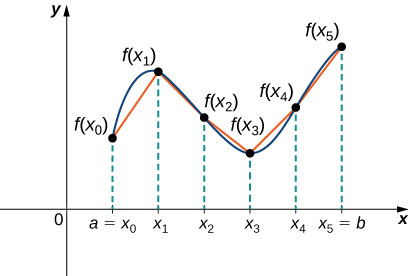
Let [latex]f(x)[/latex] be a smooth function defined over [latex]\left[a,b\right].[/latex] We want to calculate the length of the curve from the point [latex](a,f(a))[/latex] to the point [latex](b,f(b)).[/latex] We start by using line segments to approximate the length of the curve. For [latex]i=0,1,2\text{,…},n,[/latex] let [latex]P=\left\{{x}_{i}\right\}[/latex] be a regular partition of [latex]\left[a,b\right].[/latex] Then, for [latex]i=1,2\text{,…},n,[/latex] construct a line segment from the point [latex]({x}_{i-1},f({x}_{i-1}))[/latex] to the point [latex]({x}_{i},f({x}_{i})).[/latex] Although it might seem logical to use either horizontal or vertical line segments, we want our line segments to approximate the curve as closely as possible. (Figure) depicts this construct for [latex]n=5.[/latex]
To help us find the length of each line segment, we look at the change in vertical distance as well as the change in horizontal distance over each interval. Because we have used a regular partition, the change in horizontal distance over each interval is given by [latex]\text{Δ}x.[/latex] The change in vertical distance varies from interval to interval, though, so we use [latex]\text{Δ}{y}_{i}=f({x}_{i})-f({x}_{i-1})[/latex] to represent the change in vertical distance over the interval [latex]\left[{x}_{i-1},{x}_{i}\right],[/latex] as shown in (Figure). Note that some (or all) [latex]\text{Δ}{y}_{i}[/latex] may be negative.
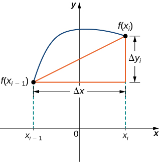
By the Pythagorean theorem, the length of the line segment is [latex]\sqrt{{(\text{Δ}x)}^{2}+{(\text{Δ}{y}_{i})}^{2}}.[/latex] We can also write this as [latex]\text{Δ}x\sqrt{1+{((\text{Δ}{y}_{i})\text{/}(\text{Δ}x))}^{2}}.[/latex] Now, by the Mean Value Theorem, there is a point [latex]{x}_{i}^{*}\in \left[{x}_{i-1},{x}_{i}\right][/latex] such that [latex]{f}^{\prime }({x}_{i}^{*})=(\text{Δ}{y}_{i})\text{/}(\text{Δ}x).[/latex] Then the length of the line segment is given by [latex]\text{Δ}x\sqrt{1+{\left[{f}^{\prime }({x}_{i}^{*})\right]}^{2}}.[/latex] Adding up the lengths of all the line segments, we get
This is a Riemann sum. Taking the limit as [latex]n\to \infty ,[/latex] we have
We summarize these findings in the following theorem.
Arc Length for [latex]y[/latex] = [latex]f[/latex]([latex]x[/latex])
Let [latex]f(x)[/latex] be a smooth function over the interval [latex]\left[a,b\right].[/latex] Then the arc length of the portion of the graph of [latex]f(x)[/latex] from the point [latex](a,f(a))[/latex] to the point [latex](b,f(b))[/latex] is given by
Note that we are integrating an expression involving [latex]{f}^{\prime }(x),[/latex] so we need to be sure [latex]{f}^{\prime }(x)[/latex] is integrable. This is why we require [latex]f(x)[/latex] to be smooth. The following example shows how to apply the theorem.
Calculating the Arc Length of a Function of [latex]x[/latex]
Let [latex]f(x)=2{x}^{3\text{/}2}.[/latex] Calculate the arc length of the graph of [latex]f(x)[/latex] over the interval [latex]\left[0,1\right].[/latex] Round the answer to three decimal places.
Let [latex]f(x)=(4\text{/}3){x}^{3\text{/}2}.[/latex] Calculate the arc length of the graph of [latex]f(x)[/latex] over the interval [latex]\left[0,1\right].[/latex] Round the answer to three decimal places.
Although it is nice to have a formula for calculating arc length, this particular theorem can generate expressions that are difficult to integrate. We study some techniques for integration in Introduction to Techniques of Integration in the second volume of this text. In some cases, we may have to use a computer or calculator to approximate the value of the integral.
Using a Computer or Calculator to Determine the Arc Length of a Function of [latex]x[/latex]
Let [latex]f(x)={x}^{2}.[/latex] Calculate the arc length of the graph of [latex]f(x)[/latex] over the interval [latex]\left[1,3\right].[/latex]
Let [latex]f(x)= \sin x.[/latex] Calculate the arc length of the graph of [latex]f(x)[/latex] over the interval [latex]\left[0,\pi \right].[/latex] Use a computer or calculator to approximate the value of the integral.
Hint
Use the process from the previous example.
Arc Length of the Curve [latex]x[/latex] = [latex]g[/latex]([latex]y[/latex])
We have just seen how to approximate the length of a curve with line segments. If we want to find the arc length of the graph of a function of [latex]y,[/latex] we can repeat the same process, except we partition the [latex]y\text{-axis}[/latex] instead of the [latex]x\text{-axis}.[/latex] (Figure) shows a representative line segment.
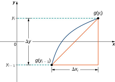
Then the length of the line segment is [latex]\sqrt{{(\text{Δ}y)}^{2}+{(\text{Δ}{x}_{i})}^{2}},[/latex] which can also be written as [latex]\text{Δ}y\sqrt{1+{((\text{Δ}{x}_{i})\text{/}(\text{Δ}y))}^{2}}.[/latex] If we now follow the same development we did earlier, we get a formula for arc length of a function [latex]x=g(y).[/latex]
Arc Length for [latex]x[/latex] = [latex]g[/latex]([latex]y[/latex])
Let [latex]g(y)[/latex] be a smooth function over an interval [latex]\left[c,d\right].[/latex] Then, the arc length of the graph of [latex]g(y)[/latex] from the point [latex](c,g(c))[/latex] to the point [latex](d,g(d))[/latex] is given by
Calculating the Arc Length of a Function of [latex]y[/latex]
Let [latex]g(y)=3{y}^{3}.[/latex] Calculate the arc length of the graph of [latex]g(y)[/latex] over the interval [latex]\left[1,2\right].[/latex]
Let [latex]g(y)=1\text{/}y.[/latex] Calculate the arc length of the graph of [latex]g(y)[/latex] over the interval [latex]\left[1,4\right].[/latex] Use a computer or calculator to approximate the value of the integral.
Hint
Use the process from the previous example.
Area of a Surface of Revolution
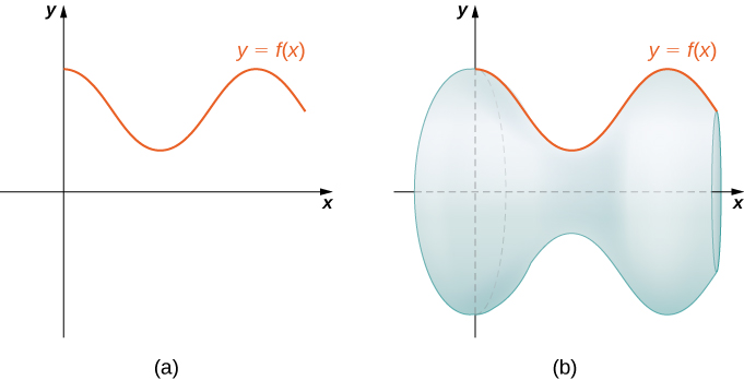
The concepts we used to find the arc length of a curve can be extended to find the surface area of a surface of revolution. Surface area is the total area of the outer layer of an object. For objects such as cubes or bricks, the surface area of the object is the sum of the areas of all of its faces. For curved surfaces, the situation is a little more complex. Let [latex]f(x)[/latex] be a nonnegative smooth function over the interval [latex]\left[a,b\right].[/latex] We wish to find the surface area of the surface of revolution created by revolving the graph of [latex]y=f(x)[/latex] around the [latex]x\text{-axis}[/latex] as shown in the following figure.
As we have done many times before, we are going to partition the interval [latex]\left[a,b\right][/latex] and approximate the surface area by calculating the surface area of simpler shapes. We start by using line segments to approximate the curve, as we did earlier in this section. For [latex]i=0,1,2\text{,…},n,[/latex] let [latex]P=\left\{{x}_{i}\right\}[/latex] be a regular partition of [latex]\left[a,b\right].[/latex] Then, for [latex]i=1,2\text{,…},n,[/latex] construct a line segment from the point [latex]({x}_{i-1},f({x}_{i-1}))[/latex] to the point [latex]({x}_{i},f({x}_{i})).[/latex] Now, revolve these line segments around the [latex]x\text{-axis}[/latex] to generate an approximation of the surface of revolution as shown in the following figure.
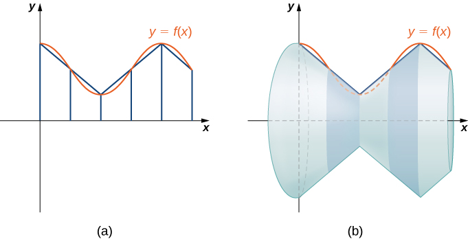
Notice that when each line segment is revolved around the axis, it produces a band. These bands are actually pieces of cones (think of an ice cream cone with the pointy end cut off). A piece of a cone like this is called a frustum of a cone.
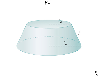
To find the surface area of the band, we need to find the lateral surface area, [latex]S,[/latex] of the frustum (the area of just the slanted outside surface of the frustum, not including the areas of the top or bottom faces). Let [latex]{r}_{1}[/latex] and [latex]{r}_{2}[/latex] be the radii of the wide end and the narrow end of the frustum, respectively, and let [latex]l[/latex] be the slant height of the frustum as shown in the following figure.
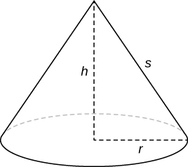
We know the lateral surface area of a cone is given by
where [latex]r[/latex] is the radius of the base of the cone and [latex]s[/latex] is the slant height (see the following figure).
Since a frustum can be thought of as a piece of a cone, the lateral surface area of the frustum is given by the lateral surface area of the whole cone less the lateral surface area of the smaller cone (the pointy tip) that was cut off (see the following figure).
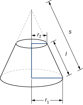
The cross-sections of the small cone and the large cone are similar triangles, so we see that
Solving for [latex]s,[/latex] we get
Then the lateral surface area (SA) of the frustum is
Let’s now use this formula to calculate the surface area of each of the bands formed by revolving the line segments around the [latex]x\text{-axis}\text{.}[/latex] A representative band is shown in the following figure.
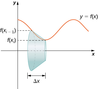
Note that the slant height of this frustum is just the length of the line segment used to generate it. So, applying the surface area formula, we have
Now, as we did in the development of the arc length formula, we apply the Mean Value Theorem to select [latex]{x}_{i}^{*}\in \left[{x}_{i-1},{x}_{i}\right][/latex] such that [latex]{f}^{\prime }({x}_{i}^{*})=(\text{Δ}{y}_{i})\text{/}\text{Δ}x.[/latex] This gives us
Furthermore, since [latex]f(x)[/latex] is continuous, by the Intermediate Value Theorem, there is a point [latex]{x}_{i}^{**}\in \left[{x}_{i-1},{x}_{i}\right][/latex] such that [latex]f({x}_{i}^{**})=(1\text{/}2)\left[f({x}_{i-1})+f({x}_{i})\right],[/latex] so we get
Then the approximate surface area of the whole surface of revolution is given by
This almost looks like a Riemann sum, except we have functions evaluated at two different points, [latex]{x}_{i}^{*}[/latex] and [latex]{x}_{i}^{**},[/latex] over the interval [latex]\left[{x}_{i-1},{x}_{i}\right].[/latex] Although we do not examine the details here, it turns out that because [latex]f(x)[/latex] is smooth, if we let [latex]n\to \infty ,[/latex] the limit works the same as a Riemann sum even with the two different evaluation points. This makes sense intuitively. Both [latex]{x}_{i}^{*}[/latex] and [latex]{x}_{i}^{**}[/latex] are in the interval [latex]\left[{x}_{i-1},{x}_{i}\right],[/latex] so it makes sense that as [latex]n\to \infty ,[/latex] both [latex]{x}_{i}^{*}[/latex] and [latex]{x}_{i}^{**}[/latex] approach [latex]x.[/latex] Those of you who are interested in the details should consult an advanced calculus text.
Taking the limit as [latex]n\to \infty ,[/latex] we get
As with arc length, we can conduct a similar development for functions of [latex]y[/latex] to get a formula for the surface area of surfaces of revolution about the [latex]y\text{-axis}.[/latex] These findings are summarized in the following theorem.
Surface Area of a Surface of Revolution
Let [latex]f(x)[/latex] be a nonnegative smooth function over the interval [latex]\left[a,b\right].[/latex] Then, the surface area of the surface of revolution formed by revolving the graph of [latex]f(x)[/latex] around the [latex]x[/latex]-axis is given by
Similarly, let [latex]g(y)[/latex] be a nonnegative smooth function over the interval [latex]\left[c,d\right].[/latex] Then, the surface area of the surface of revolution formed by revolving the graph of [latex]g(y)[/latex] around the [latex]y\text{-axis}[/latex] is given by
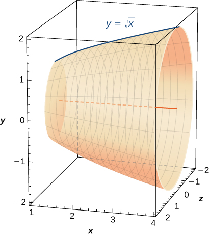
Calculating the Surface Area of a Surface of Revolution 1
Let [latex]f(x)=\sqrt{x}[/latex] over the interval [latex]\left[1,4\right].[/latex] Find the surface area of the surface generated by revolving the graph of [latex]f(x)[/latex] around the [latex]x\text{-axis}.[/latex] Round the answer to three decimal places.

Let [latex]f(x)=\sqrt{1-x}[/latex] over the interval [latex]\left[0,1\text{/}2\right].[/latex] Find the surface area of the surface generated by revolving the graph of [latex]f(x)[/latex] around the [latex]x\text{-axis}.[/latex] Round the answer to three decimal places.
Hint
Use the process from the previous example.
Calculating the Surface Area of a Surface of Revolution 2
Let [latex]f(x)=y=\sqrt[3]{3x}.[/latex] Consider the portion of the curve where [latex]0\le y\le 2.[/latex] Find the surface area of the surface generated by revolving the graph of [latex]f(x)[/latex] around the [latex]y\text{-axis}.[/latex]

Let [latex]g(y)=\sqrt{9-{y}^{2}}[/latex] over the interval [latex]y\in \left[0,2\right].[/latex] Find the surface area of the surface generated by revolving the graph of [latex]g(y)[/latex] around the [latex]y\text{-axis}.[/latex]
Hint
Use the process from the previous example.
Key Concepts
- The arc length of a curve can be calculated using a definite integral.
- The arc length is first approximated using line segments, which generates a Riemann sum. Taking a limit then gives us the definite integral formula. The same process can be applied to functions of [latex]y.[/latex]
- The concepts used to calculate the arc length can be generalized to find the surface area of a surface of revolution.
- The integrals generated by both the arc length and surface area formulas are often difficult to evaluate. It may be necessary to use a computer or calculator to approximate the values of the integrals.
Key Equations
- Arc Length of a Function of [latex]x[/latex]
[latex]\text{Arc Length}={\int }_{a}^{b}\sqrt{1+{\left[{f}^{\prime }(x)\right]}^{2}}dx[/latex] - Arc Length of a Function of [latex]y[/latex]
[latex]\text{Arc Length}={\int }_{c}^{d}\sqrt{1+{\left[{g}^{\prime }(y)\right]}^{2}}dy[/latex] - Surface Area of a Function of [latex]x[/latex]
[latex]\text{Surface Area}={\int }_{a}^{b}(2\pi f(x)\sqrt{1+{({f}^{\prime }(x))}^{2}})dx[/latex]
For the following exercises, find the length of the functions over the given interval.
1. [latex]y=5x\text{from}x=0\text{ to }x=2[/latex]
2. [latex]y=-\frac{1}{2}x+25\text{from}x=1\text{ to }x=4[/latex]
3. [latex]x=4y\text{from}y=-1\text{ to }y=1[/latex]
4. Pick an arbitrary linear function [latex]x=g(y)[/latex] over any interval of your choice [latex]({y}_{1},{y}_{2}).[/latex] Determine the length of the function and then prove the length is correct by using geometry.
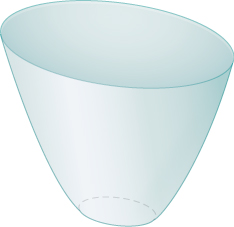
5. Find the surface area of the volume generated when the curve [latex]y=\sqrt{x}[/latex] revolves around the [latex]x\text{-axis}[/latex] from [latex](1,1)[/latex] to [latex](4,2),[/latex] as seen here.
6. Find the surface area of the volume generated when the curve [latex]y={x}^{2}[/latex] revolves around the [latex]y\text{-axis}[/latex] from [latex](1,1)[/latex] to [latex](3,9).[/latex]
For the following exercises, find the lengths of the functions of [latex]x[/latex] over the given interval. If you cannot evaluate the integral exactly, use technology to approximate it.
7. [latex]y={x}^{3\text{/}2}[/latex] from [latex](0,0)\text{ to }(1,1)[/latex]
8. [latex]y={x}^{2\text{/}3}[/latex] from [latex](1,1)\text{ to }(8,4)[/latex]
9. [latex]y=\frac{1}{3}{({x}^{2}+2)}^{3\text{/}2}[/latex] from [latex]x=0\text{ to }x=1[/latex]
10. [latex]y=\frac{1}{3}{({x}^{2}-2)}^{3\text{/}2}[/latex] from [latex]x=2[/latex] to [latex]x=4[/latex]
11. [T][latex]y={e}^{x}[/latex] on [latex]x=0[/latex] to [latex]x=1[/latex]
12. [latex]y=\frac{{x}^{3}}{3}+\frac{1}{4x}[/latex] from [latex]x=1\text{ to }x=3[/latex]
13. [latex]y=\frac{{x}^{4}}{4}+\frac{1}{8{x}^{2}}[/latex] from [latex]x=1\text{ to }x=2[/latex]
14. [latex]y=\frac{2{x}^{3\text{/}2}}{3}-\frac{{x}^{1\text{/}2}}{2}[/latex] from [latex]x=1\text{ to }x=4[/latex]
15. [latex]y=\frac{1}{27}{(9{x}^{2}+6)}^{3\text{/}2}[/latex] from [latex]x=0\text{ to }x=2[/latex]
16. [T][latex]y= \sin x[/latex] on [latex]x=0\text{ to }x=\pi[/latex]
For the following exercises, find the lengths of the functions of [latex]y[/latex] over the given interval. If you cannot evaluate the integral exactly, use technology to approximate it.
17. [latex]y=\frac{5-3x}{4}[/latex] from [latex]y=0[/latex] to [latex]y=4[/latex]
[latex]\frac{20}{3}[/latex]
18. [latex]x=\frac{1}{2}({e}^{y}+{e}^{\text{−}y})[/latex] from [latex]y=-1\text{ to }y=1[/latex]
19. [latex]x=5{y}^{3\text{/}2}[/latex] from [latex]y=0[/latex] to [latex]y=1[/latex]
20. [T][latex]x={y}^{2}[/latex] from [latex]y=0[/latex] to [latex]y=1[/latex]
21. [latex]x=\sqrt{y}[/latex] from [latex]y=0\text{ to }y=1[/latex]
22. [latex]x=\frac{2}{3}{({y}^{2}+1)}^{3\text{/}2}[/latex] from [latex]y=1[/latex] to [latex]y=3[/latex]
23. [T][latex]x= \tan y[/latex] from [latex]y=0[/latex] to [latex]y=\frac{3}{4}[/latex]
24. [T][latex]x={ \cos }^{2}y[/latex] from [latex]y=-\frac{\pi }{2}[/latex] to [latex]y=\frac{\pi }{2}[/latex]
25. [T][latex]x={4}^{y}[/latex] from [latex]y=0\text{ to }y=2[/latex]
26. [T][latex]x=\text{ln}(y)[/latex] on [latex]y=\frac{1}{e}[/latex] to [latex]y=e[/latex]
For the following exercises, find the surface area of the volume generated when the following curves revolve around the [latex]x\text{-axis}.[/latex] If you cannot evaluate the integral exactly, use your calculator to approximate it.
27. [latex]y=\sqrt{x}[/latex] from [latex]x=2[/latex] to [latex]x=6[/latex]
28. [latex]y={x}^{3}[/latex] from [latex]x=0[/latex] to [latex]x=1[/latex]
29. [latex]y=7x[/latex] from [latex]x=-1\text{ to }x=1[/latex]
30. [T][latex]y=\frac{1}{{x}^{2}}[/latex] from [latex]x=1\text{ to }x=3[/latex]
31. [latex]y=\sqrt{4-{x}^{2}}[/latex] from [latex]x=0\text{ to }x=2[/latex]
[latex]8\pi[/latex]
32. [latex]y=\sqrt{4-{x}^{2}}[/latex] from [latex]x=-1\text{ to }x=1[/latex]
33. [latex]y=5x[/latex] from [latex]x=1\text{ to }x=5[/latex]
34. [T][latex]y= \tan x[/latex] from [latex]x=-\frac{\pi }{4}\text{ to }x=\frac{\pi }{4}[/latex]
For the following exercises, find the surface area of the volume generated when the following curves revolve around the [latex]y\text{-axis}\text{.}[/latex] If you cannot evaluate the integral exactly, use your calculator to approximate it.
35. [latex]y={x}^{2}[/latex] from [latex]x=0\text{ to }x=2[/latex]
36. [latex]y=\frac{1}{2}{x}^{2}+\frac{1}{2}[/latex] from [latex]x=0\text{ to }x=1[/latex]
37. [latex]y=x+1[/latex] from [latex]x=0\text{ to }x=3[/latex]
38. [T][latex]y=\frac{1}{x}[/latex] from [latex]x=\frac{1}{2}[/latex] to [latex]x=1[/latex]
39. [latex]y=\sqrt[3]{x}[/latex] from [latex]x=1\text{ to }x=27[/latex]
40. [T][latex]y=3{x}^{4}[/latex] from [latex]x=0[/latex] to [latex]x=1[/latex]
41. [T][latex]y=\frac{1}{\sqrt{x}}[/latex] from [latex]x=1[/latex] to [latex]x=3[/latex]
42. [T][latex]y= \cos x[/latex] from [latex]x=0[/latex] to [latex]x=\frac{\pi }{2}[/latex]
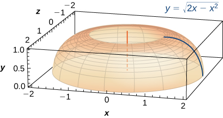
43. The base of a lamp is constructed by revolving a quarter circle [latex]y=\sqrt{2x-{x}^{2}}[/latex] around the [latex]y\text{-axis}[/latex] from [latex]x=1[/latex] to [latex]x=2,[/latex] as seen here. Create an integral for the surface area of this curve and compute it.
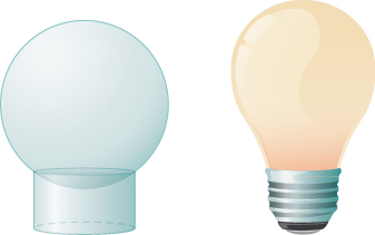
44. A light bulb is a sphere with radius [latex]1\text{/}2[/latex] in. with the bottom sliced off to fit exactly onto a cylinder of radius [latex]1\text{/}4[/latex] in. and length [latex]1\text{/}3[/latex] in., as seen here. The sphere is cut off at the bottom to fit exactly onto the cylinder, so the radius of the cut is [latex]1\text{/}4[/latex] in. Find the surface area (not including the top or bottom of the cylinder).
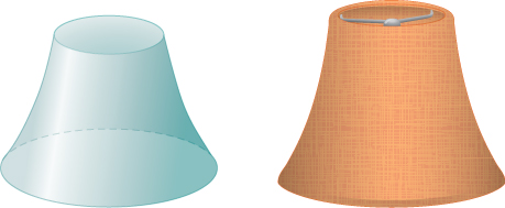
45. [T] A lampshade is constructed by rotating [latex]y=1\text{/}x[/latex] around the [latex]x\text{-axis}[/latex] from [latex]y=1[/latex] to [latex]y=2,[/latex] as seen here. Determine how much material you would need to construct this lampshade—that is, the surface area—accurate to four decimal places.
46. [T] An anchor drags behind a boat according to the function [latex]y=24{e}^{\text{−}x\text{/}2}-24,[/latex] where [latex]y[/latex] represents the depth beneath the boat and [latex]x[/latex] is the horizontal distance of the anchor from the back of the boat. If the anchor is 23 ft below the boat, how much rope do you have to pull to reach the anchor? Round your answer to three decimal places.
47. [T] You are building a bridge that will span 10 ft. You intend to add decorative rope in the shape of [latex]y=5| \sin ((x\pi )\text{/}5)|,[/latex] where [latex]x[/latex] is the distance in feet from one end of the bridge. Find out how much rope you need to buy, rounded to the nearest foot.
For the following exercises, find the exact arc length for the following problems over the given interval.
48. [latex]y=\text{ln}( \sin x)[/latex] from [latex]x=\pi \text{/}4[/latex] to [latex]x=(3\pi )\text{/}4.[/latex] (Hint: Recall trigonometric identities.)
49. Draw graphs of [latex]y={x}^{2},[/latex] [latex]y={x}^{6},[/latex] and [latex]y={x}^{10}.[/latex] For [latex]y={x}^{n},[/latex] as [latex]n[/latex] increases, formulate a prediction on the arc length from [latex](0,0)[/latex] to [latex](1,1).[/latex] Now, compute the lengths of these three functions and determine whether your prediction is correct.
50. Compare the lengths of the parabola [latex]x={y}^{2}[/latex] and the line [latex]x=by[/latex] from [latex](0,0)\text{ to }({b}^{2},b)[/latex] as [latex]b[/latex] increases. What do you notice?
51. Solve for the length of [latex]x={y}^{2}[/latex] from [latex](0,0)\text{ to }(1,1).[/latex] Show that [latex]x=(1\text{/}2){y}^{2}[/latex] from [latex](0,0)[/latex] to [latex](2,2)[/latex] is twice as long. Graph both functions and explain why this is so.
52. [T] Which is longer between [latex](1,1)[/latex] and [latex](2,1\text{/}2)\text{:}[/latex] the hyperbola [latex]y=1\text{/}x[/latex] or the graph of [latex]x+2y=3?[/latex]
54. Explain why the surface area is infinite when [latex]y=1\text{/}x[/latex] is rotated around the [latex]x\text{-axis}[/latex] for [latex]1\le x<\infty ,[/latex] but the volume is finite.
Glossary
- arc length
- the arc length of a curve can be thought of as the distance a person would travel along the path of the curve
- frustum
- a portion of a cone; a frustum is constructed by cutting the cone with a plane parallel to the base
- surface area
- the surface area of a solid is the total area of the outer layer of the object; for objects such as cubes or bricks, the surface area of the object is the sum of the areas of all of its faces
Candela Citations
- Calculus I. Provided by: OpenStax. Located at: http://cnx.org/contents/8b89d172-2927-466f-8661-01abc7ccdba4@2.89. License: CC BY-NC-SA: Attribution-NonCommercial-ShareAlike. License Terms: Download for free at http://cnx.org/contents/8b89d172-2927-466f-8661-01abc7ccdba4@2.89

Hint
Use the process from the previous example. Don’t forget to change the limits of integration.