Learning Objectives
- Describe the steps of Newton’s method.
- Explain what an iterative process means.
- Recognize when Newton’s method does not work.
- Apply iterative processes to various situations.
In many areas of pure and applied mathematics, we are interested in finding solutions to an equation of the form [latex]f(x)=0[/latex]. For most functions, however, it is difficult—if not impossible—to calculate their zeroes explicitly. In this section, we take a look at a technique that provides a very efficient way of approximating the zeroes of functions. This technique makes use of tangent line approximations and is behind the method used often by calculators and computers to find zeroes.
Describing Newton’s Method
Consider the task of finding the solutions of [latex]f(x)=0[/latex]. If [latex]f[/latex] is the first-degree polynomial [latex]f(x)=ax+b[/latex], then the solution of [latex]f(x)=0[/latex] is given by the formula [latex]x=-\frac{b}{a}[/latex]. If [latex]f[/latex] is the second-degree polynomial [latex]f(x)=ax^2+bx+c[/latex], the solutions of [latex]f(x)=0[/latex] can be found by using the quadratic formula. However, for polynomials of degree 3 or more, finding roots of [latex]f[/latex] becomes more complicated. Although formulas exist for third- and fourth-degree polynomials, they are quite complicated. Also, if [latex]f[/latex] is a polynomial of degree 5 or greater, it is known that no such formulas exist. For example, consider the function
No formula exists that allows us to find the solutions of [latex]f(x)=0[/latex]. Similar difficulties exist for nonpolynomial functions. For example, consider the task of finding solutions of [latex]\tan (x)-x=0[/latex]. No simple formula exists for the solutions of this equation. In cases such as these, we can use Newton’s method to approximate the roots.
Newton’s method makes use of the following idea to approximate the solutions of [latex]f(x)=0[/latex]. By sketching a graph of [latex]f[/latex], we can estimate a root of [latex]f(x)=0[/latex]. Let’s call this estimate [latex]x_0[/latex]. We then draw the tangent line to [latex]f[/latex] at [latex]x_0[/latex]. If [latex]f^{\prime}(x_0)\ne 0[/latex], this tangent line intersects the [latex]x[/latex]-axis at some point [latex](x_1,0)[/latex]. Now let [latex]x_1[/latex] be the next approximation to the actual root. Typically, [latex]x_1[/latex] is closer than [latex]x_0[/latex] to an actual root. Next we draw the tangent line to [latex]f[/latex] at [latex]x_1[/latex]. If [latex]f^{\prime}(x_1)\ne 0[/latex], this tangent line also intersects the [latex]x[/latex]-axis, producing another approximation, [latex]x_2[/latex]. We continue in this way, deriving a list of approximations: [latex]x_0, x_1, x_2, \cdots[/latex]. Typically, the numbers [latex]x_0,x_1,x_2, \cdots[/latex] quickly approach an actual root [latex]x*[/latex], as shown in the following figure.
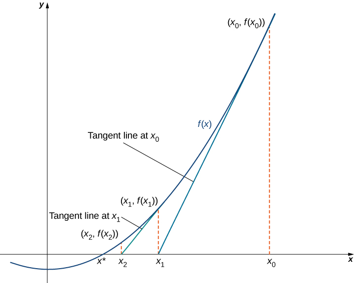
Figure 1. The approximations [latex]x_0,x_1,x_2, \cdots[/latex] approach the actual root [latex]x*[/latex]. The approximations are derived by looking at tangent lines to the graph of [latex]f[/latex].
Now let’s look at how to calculate the approximations [latex]x_0,x_1,x_2, \cdots[/latex]. If [latex]x_0[/latex] is our first approximation, the approximation [latex]x_1[/latex] is defined by letting [latex](x_1,0)[/latex] be the [latex]x[/latex]-intercept of the tangent line to [latex]f[/latex] at [latex]x_0[/latex]. The equation of this tangent line is given by
Therefore, [latex]x_1[/latex] must satisfy
Solving this equation for [latex]x_1[/latex], we conclude that
Similarly, the point [latex](x_2,0)[/latex] is the [latex]x[/latex]-intercept of the tangent line to [latex]f[/latex] at [latex]x_1[/latex]. Therefore, [latex]x_2[/latex] satisfies the equation
In general, for [latex]n>0, \, x_n[/latex] satisfies
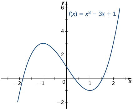
Next we see how to make use of this technique to approximate the root of the polynomial [latex]f(x)=x^3-3x+1[/latex].
Finding a Root of a Polynomial
Use Newton’s method to approximate a root of [latex]f(x)=x^3-3x+1[/latex] in the interval [latex][1,2][/latex]. Let [latex]x_0=2[/latex] and find [latex]x_1,x_2,x_3,x_4[/latex], and [latex]x_5[/latex].
Letting [latex]x_0=0[/latex], use Newton’s method to approximate the root of [latex]f(x)=x^3-3x+1[/latex] over the interval [latex][0,1][/latex] by calculating [latex]x_1[/latex] and [latex]x_2[/latex].
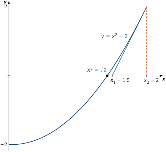
Newton’s method can also be used to approximate square roots. Here we show how to approximate [latex]\sqrt{2}[/latex]. This method can be modified to approximate the square root of any positive number.
Finding a Square Root
Use Newton’s method to approximate [latex]\sqrt{2}[/latex] ((Figure)). Let [latex]f(x)=x^2-2[/latex], let [latex]x_0=2[/latex], and calculate [latex]x_1,x_2,x_3,x_4,x_5[/latex]. (We note that since [latex]f(x)=x^2-2[/latex] has a zero at [latex]\sqrt{2}[/latex], the initial value [latex]x_0=2[/latex] is a reasonable choice to approximate [latex]\sqrt{2}[/latex].)
Use Newton’s method to approximate [latex]\sqrt{3}[/latex] by letting [latex]f(x)=x^2-3[/latex] and [latex]x_0=3[/latex]. Find [latex]x_1[/latex] and [latex]x_2[/latex].
Hint
For [latex]f(x)=x^2-3[/latex], (Figure) reduces to [latex]x_n=\frac{x_{n-1}}{2}+\frac{3}{2x_{n-1}}[/latex].
When using Newton’s method, each approximation after the initial guess is defined in terms of the previous approximation by using the same formula. In particular, by defining the function [latex]F(x)=x-[\frac{f(x)}{f^{\prime}(x)}][/latex], we can rewrite (Figure) as [latex]x_n=F(x_{n-1})[/latex]. This type of process, where each [latex]x_n[/latex] is defined in terms of [latex]x_{n-1}[/latex] by repeating the same function, is an example of an iterative process. Shortly, we examine other iterative processes. First, let’s look at the reasons why Newton’s method could fail to find a root.
Failures of Newton’s Method
Typically, Newton’s method is used to find roots fairly quickly. However, things can go wrong. Some reasons why Newton’s method might fail include the following:
- At one of the approximations [latex]x_n[/latex], the derivative [latex]f^{\prime}[/latex] is zero at [latex]x_n[/latex], but [latex]f(x_n) \ne 0[/latex]. As a result, the tangent line of [latex]f[/latex] at [latex]x_n[/latex] does not intersect the [latex]x[/latex]-axis. Therefore, we cannot continue the iterative process.
- The approximations [latex]x_0,x_1,x_2, \cdots[/latex] may approach a different root. If the function [latex]f[/latex] has more than one root, it is possible that our approximations do not approach the one for which we are looking, but approach a different root (see (Figure)). This event most often occurs when we do not choose the approximation [latex]x_0[/latex] close enough to the desired root.
- The approximations may fail to approach a root entirely. In (Figure), we provide an example of a function and an initial guess [latex]x_0[/latex] such that the successive approximations never approach a root because the successive approximations continue to alternate back and forth between two values.
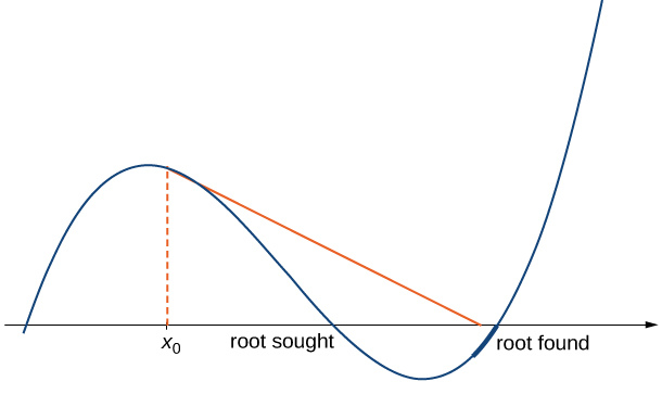
Figure 4. If the initial guess [latex]x_0[/latex] is too far from the root sought, it may lead to approximations that approach a different root.
When Newton’s Method Fails
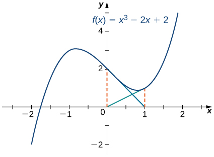
Consider the function [latex]f(x)=x^3-2x+2[/latex]. Let [latex]x_0=0[/latex]. Show that the sequence [latex]x_1,x_2, \cdots[/latex] fails to approach a root of [latex]f[/latex].
For [latex]f(x)=x^3-2x+2[/latex], let [latex]x_0=-1.5[/latex] and find [latex]x_1[/latex] and [latex]x_2[/latex].
Hint
Use (Figure).
From (Figure), we see that Newton’s method does not always work. However, when it does work, the sequence of approximations approaches the root very quickly. Discussions of how quickly the sequence of approximations approach a root found using Newton’s method are included in texts on numerical analysis.
Other Iterative Processes
As mentioned earlier, Newton’s method is a type of iterative process. We now look at an example of a different type of iterative process.
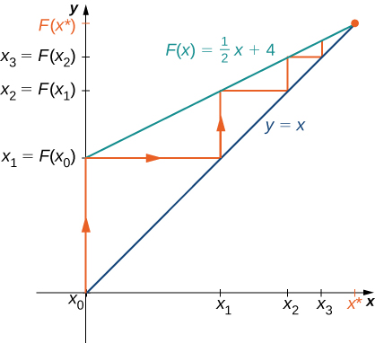
Consider a function [latex]F[/latex] and an initial number [latex]x_0[/latex]. Define the subsequent numbers [latex]x_n[/latex] by the formula [latex]x_n=F(x_{n-1})[/latex]. This process is an iterative process that creates a list of numbers [latex]x_0,x_1,x_2, \cdots ,x_n, \cdots[/latex]. This list of numbers may approach a finite number [latex]x*[/latex] as [latex]n[/latex] gets larger, or it may not. In (Figure), we see an example of a function [latex]F[/latex] and an initial guess [latex]x_0[/latex] such that the resulting list of numbers approaches a finite value.
Finding a Limit for an Iterative Process
Let [latex]F(x)=\frac{1}{2}x+4[/latex] and let [latex]x_0=0[/latex]. For all [latex]n \ge 1[/latex], let [latex]x_n=F(x_{n-1})[/latex]. Find the values [latex]x_1,x_2,x_3,x_4,x_5[/latex]. Make a conjecture about what happens to this list of numbers [latex]x_1,x_2,x_3, \cdots,x_n, \cdots[/latex] as [latex]n\to \infty[/latex]. If the list of numbers [latex]x_1,x_2,x_3, \cdots[/latex] approaches a finite number [latex]x^*[/latex], then [latex]x^*[/latex] satisfies [latex]x^*=F(x^*)[/latex], and [latex]x^*[/latex] is called a fixed point of [latex]F[/latex].
Consider the function [latex]F(x)=\frac{1}{3}x+6[/latex]. Let [latex]x_0=0[/latex] and let [latex]x_n=F(x_{n-1})[/latex] for [latex]n \ge 2[/latex]. Find [latex]x_1,x_2,x_3,x_4,x_5[/latex]. Make a conjecture about what happens to the list of numbers [latex]x_1,x_2,x_3, \cdots, x_n, \cdots[/latex] as [latex]n\to \infty[/latex].
Hint
Consider the point where the lines [latex]y=x[/latex] and [latex]y=F(x)[/latex] intersect.
Student Project: Iterative Processes and Chaos
Iterative processes can yield some very interesting behavior. In this section, we have seen several examples of iterative processes that converge to a fixed point. We also saw in (Figure) that the iterative process bounced back and forth between two values. We call this kind of behavior a 2-cycle. Iterative processes can converge to cycles with various periodicities, such as 2-cycles, 4-cycles (where the iterative process repeats a sequence of four values), 8-cycles, and so on.
Some iterative processes yield what mathematicians call chaos. In this case, the iterative process jumps from value to value in a seemingly random fashion and never converges or settles into a cycle. Although a complete exploration of chaos is beyond the scope of this text, in this project we look at one of the key properties of a chaotic iterative process: sensitive dependence on initial conditions. This property refers to the concept that small changes in initial conditions can generate drastically different behavior in the iterative process.
Probably the best-known example of chaos is the Mandelbrot set (see (Figure)), named after Benoit Mandelbrot (1924–2010), who investigated its properties and helped popularize the field of chaos theory. The Mandelbrot set is usually generated by computer and shows fascinating details on enlargement, including self-replication of the set. Several colorized versions of the set have been shown in museums and can be found online and in popular books on the subject.

Figure 7. The Mandelbrot set is a well-known example of a set of points generated by the iterative chaotic behavior of a relatively simple function.
In this project we use the logistic map
as the function in our iterative process. The logistic map is a deceptively simple function; but, depending on the value of [latex]r[/latex], the resulting iterative process displays some very interesting behavior. It can lead to fixed points, cycles, and even chaos.
To visualize the long-term behavior of the iterative process associated with the logistic map, we will use a tool called a cobweb diagram. As we did with the iterative process we examined earlier in this section, we first draw a vertical line from the point [latex](x_0,0)[/latex] to the point [latex](x_0,f(x_0))=(x_0,x_1)[/latex]. We then draw a horizontal line from that point to the point [latex](x_1,x_1)[/latex], then draw a vertical line to [latex](x_1,f(x_1))=(x_1,x_2)[/latex], and continue the process until the long-term behavior of the system becomes apparent. (Figure) shows the long-term behavior of the logistic map when [latex]r=3.55[/latex] and [latex]x_0=0.2[/latex]. (The first 100 iterations are not plotted.) The long-term behavior of this iterative process is an 8-cycle.
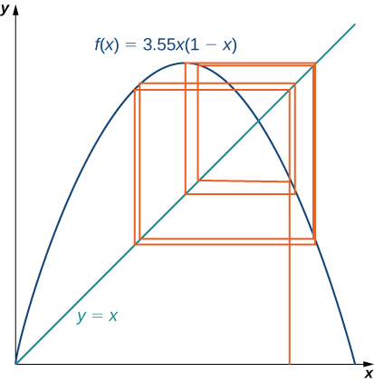
Figure 8. A cobweb diagram for [latex]f(x)=3.55x(1-x)[/latex] is presented here. The sequence of values results in an 8-cycle.
- Let [latex]r=0.5[/latex] and choose [latex]x_0=0.2[/latex]. Either by hand or by using a computer, calculate the first 10 values in the sequence. Does the sequence appear to converge? If so, to what value? Does it result in a cycle? If so, what kind of cycle (for example, 2-cycle, 4-cycle)?
- What happens when [latex]r=2[/latex]?
- For [latex]r=3.2[/latex] and [latex]r=3.5[/latex], calculate the first 100 sequence values. Generate a cobweb diagram for each iterative process. (Several free applets are available online that generate cobweb diagrams for the logistic map.) What is the long-term behavior in each of these cases?
- Now let [latex]r=4[/latex]. Calculate the first 100 sequence values and generate a cobweb diagram. What is the long-term behavior in this case?
- Repeat the process for [latex]r=4[/latex], but let [latex]x_0=0.201[/latex]. How does this behavior compare with the behavior for [latex]x_0=0.2[/latex]?
Key Concepts
- Newton’s method approximates roots of [latex]f(x)=0[/latex] by starting with an initial approximation [latex]x_0[/latex], then uses tangent lines to the graph of [latex]f[/latex] to create a sequence of approximations [latex]x_1,x_2,x_3, \cdots[/latex].
- Typically, Newton’s method is an efficient method for finding a particular root. In certain cases, Newton’s method fails to work because the list of numbers [latex]x_0,x_1,x_2, \cdots[/latex] does not approach a finite value or it approaches a value other than the root sought.
- Any process in which a list of numbers [latex]x_0,x_1,x_2, \cdots[/latex] is generated by defining an initial number [latex]x_0[/latex] and defining the subsequent numbers by the equation [latex]x_n=F(x_{n-1})[/latex] for some function [latex]F[/latex] is an iterative process. Newton’s method is an example of an iterative process, where the function [latex]F(x)=x-[\frac{f(x)}{f^{\prime}(x)}][/latex] for a given function [latex]f[/latex].
For the following exercises, write Newton’s formula as [latex]x_{n+1}=F(x_n)[/latex] for solving [latex]f(x)=0[/latex].
1. [latex]f(x)=x^2+1[/latex]
2. [latex]f(x)=x^3+2x+1[/latex]
3. [latex]f(x)= \sin x[/latex]
4. [latex]f(x)=e^x[/latex]
5. [latex]f(x)=x^3+3xe^x[/latex]
For the following exercises, solve [latex]f(x)=0[/latex] using the iteration [latex]x_{n+1}=x_n-cf(x_n)[/latex], which differs slightly from Newton’s method. Find a [latex]c[/latex] that works and a [latex]c[/latex] that fails to converge, with the exception of [latex]c=0[/latex].
6. [latex]f(x)=x^2-4[/latex], with [latex]x_0=0[/latex]
7. [latex]f(x)=x^2-4x+3[/latex], with [latex]x_0=2[/latex]
8. What is the value of “[latex]c[/latex]” for Newton’s method?
For the following exercises, start at
a. [latex]x_0=0.6[/latex] and
b. [latex]x_0=2[/latex].
Compute [latex]x_1[/latex] and [latex]x_2[/latex] using the specified iterative method.
9. [latex]x_{n+1}=(x_n)^2-\frac{1}{2}[/latex]
10. [latex]x_{n+1}=2x_n(1-x_n)[/latex]
11. [latex]x_{n+1}=\sqrt{x_n}[/latex]
12. [latex]x_{n+1}=\frac{1}{\sqrt{x_n}}[/latex]
13. [latex]x_{n+1}=3x_n(1-x_n)[/latex]
14. [latex]x_{n+1}=(x_n)^2+x_n-2[/latex]
15. [latex]x_{n+1}=\frac{1}{2}x_n-1[/latex]
16. [latex]x_{n+1}=|x_n|[/latex]
For the following exercises, solve to four decimal places using Newton’s method and a computer or calculator. Choose any initial guess [latex]x_0[/latex] that is not the exact root.
17. [latex]x^2-10=0[/latex]
18. [latex]x^4-100=0[/latex]
19. [latex]x^2-x=0[/latex]
20.[latex]x^3-x=0[/latex]
21. [latex]x+5 \cos (x)=0[/latex]
22. [latex]x+ \tan (x)=0[/latex], choose [latex]x_0 \in (-\frac{\pi}{2},\frac{\pi }{2})[/latex]
23. [latex]\frac{1}{1-x}=2[/latex]
24. [latex]1+x+x^2+x^3+x^4=2[/latex]
25. [latex]x^3+(x+1)^3=10^3[/latex]
26. [latex]x= \sin^2 (x)[/latex]
For the following exercises, use Newton’s method to find the fixed points of the function where [latex]f(x)=x[/latex]; round to three decimals.
27. [latex]\sin x[/latex]
28. [latex]\tan (x)[/latex] on [latex]x \in (\frac{\pi }{2},\frac{3\pi }{2})[/latex]
29. [latex]e^x-2[/latex]
30. [latex]\ln (x)+2[/latex]
Newton’s method can be used to find maxima and minima of functions in addition to the roots. In this case apply Newton’s method to the derivative function [latex]f^{\prime}(x)[/latex] to find its roots, instead of the original function. For the following exercises, consider the formulation of the method.
31. To find candidates for maxima and minima, we need to find the critical points [latex]f^{\prime}(x)=0[/latex]. Show that to solve for the critical points of a function [latex]f(x)[/latex], Newton’s method is given by [latex]x_{n+1}=x_n-\frac{f^{\prime}(x_n)}{f^{\prime \prime}(x_n)}[/latex].
32. What additional restrictions are necessary on the function [latex]f[/latex]?
For the following exercises, use Newton’s method to find the location of the local minima and/or maxima of the following functions; round to three decimals.
33. Minimum of [latex]f(x)=x^2+2x+4[/latex]
34. Minimum of [latex]f(x)=3x^3+2x^2-16[/latex]
35. Minimum of [latex]f(x)=x^2e^x[/latex]
36. Maximum of [latex]f(x)=x+\frac{1}{x}[/latex]
37. Maximum of [latex]f(x)=x^3+10x^2+15x-2[/latex]
38. Maximum of [latex]f(x)=\frac{\sqrt{x}-\sqrt[3]{x}}{x}[/latex]
39. Minimum of [latex]f(x)=x^2 \sin x[/latex], closest non-zero minimum to [latex]x=0[/latex]
40. Minimum of [latex]f(x)=x^4+x^3+3x^2+12x+6[/latex]
For the following exercises, use the specified method to solve the equation. If it does not work, explain why it does not work.
41. Newton’s method, [latex]x^2+2=0[/latex]
42. Newton’s method, [latex]0=e^x[/latex]
43. Newton’s method, [latex]0=1+x^2[/latex] starting at [latex]x_0=0[/latex]
44. Solving [latex]x_{n+1}=−(x_n)^3[/latex] starting at [latex]x_0=-1[/latex]
For the following exercises, use the secant method, an alternative iterative method to Newton’s method. The formula is given by
45. Find a root to [latex]0=x^2-x-3[/latex] accurate to three decimal places.
46. Find a root to [latex]0= \sin x+3x[/latex] accurate to four decimal places.
47. Find a root to [latex]0=e^x-2[/latex] accurate to four decimal places.
48. Find a root to [latex]\ln (x+2)=\frac{1}{2}[/latex] accurate to four decimal places.
49. Why would you use the secant method over Newton’s method? What are the necessary restrictions on [latex]f[/latex]?
For the following exercises, use both Newton’s method and the secant method to calculate a root for the following equations. Use a calculator or computer to calculate how many iterations of each are needed to reach within three decimal places of the exact answer. For the secant method, use the first guess from Newton’s method.
50. [latex]f(x)=x^2+2x+1, \, x_0=1[/latex]
51. [latex]f(x)=x^2, \, x_0=1[/latex]
52. [latex]f(x)= \sin x, \, x_0=1[/latex]
53. [latex]f(x)=e^x-1, \, x_0=2[/latex]
54. [latex]f(x)=x^3+2x+4, \, x_0=0[/latex]
In the following exercises, consider Kepler’s equation regarding planetary orbits, [latex]M=E-\epsilon \sin (E)[/latex], where [latex]M[/latex] is the mean anomaly, [latex]E[/latex] is eccentric anomaly, and [latex]\epsilon[/latex] measures eccentricity.
55. Use Newton’s method to solve for the eccentric anomaly [latex]E[/latex] when the mean anomaly [latex]M=\frac{\pi }{3}[/latex] and the eccentricity of the orbit [latex]\epsilon =0.25[/latex]; round to three decimals.
56. Use Newton’s method to solve for the eccentric anomaly [latex]E[/latex] when the mean anomaly [latex]M=\frac{3\pi }{2}[/latex] and the eccentricity of the orbit [latex]\epsilon =0.8[/latex]; round to three decimals.
The following two exercises consider a bank investment. The initial investment is [latex]$10,000[/latex]. After 25 years, the investment has tripled to [latex]$30,000[/latex].
57. Use Newton’s method to determine the interest rate if the interest was compounded annually.
58. Use Newton’s method to determine the interest rate if the interest was compounded continuously.
59. The cost for printing a book can be given by the equation [latex]C(x)=1000+12x+(\frac{1}{2})x^{2/3}[/latex]. Use Newton’s method to find the break-even point if the printer sells each book for [latex]$20[/latex].
Glossary
- iterative process
- process in which a list of numbers [latex]x_0,x_1,x_2,x_3, \cdots[/latex] is generated by starting with a number [latex]x_0[/latex] and defining [latex]x_n=F(x_{n-1})[/latex] for [latex]n \ge 1[/latex]
- Newton’s method
- method for approximating roots of [latex]f(x)=0[/latex]; using an initial guess [latex]x_0[/latex], each subsequent approximation is defined by the equation [latex]x_n=x_{n-1}-\frac{f(x_{n-1})}{f^{\prime}(x_{n-1})}[/latex]
Candela Citations
- Calculus I. Provided by: OpenStax. Located at: http://cnx.org/contents/8b89d172-2927-466f-8661-01abc7ccdba4@2.89. License: CC BY-NC-SA: Attribution-NonCommercial-ShareAlike. License Terms: Download for free at http://cnx.org/contents/8b89d172-2927-466f-8661-01abc7ccdba4@2.89

Hint
Use (Figure).