M. Affan Badar, Shyamsundarreddy Sammidi, and Leslie Gardner’s “Reducing the Bullwhip Effect in the Supply Chain: A Study of Different Ordering Strategies”
Read this article. The costs of the supply chain can have a negative effect on the organization’s profitability. This is important because we must make wise choices when choosing the strategy to manage the supply chain. As you read, consider the importance of controlling the ordering strategy of the company.
Reducing the Bullwhip Effect in the Supply Chain: A Study of Different Ordering Strategies
Abstract
Profitability of a company can be affected by the costs associated with backlogs and large inventories due to the bullwhip effect in the supply chain. This work aims to find an ordering strategy that is practical and can minimize the bullwhip effect. Five strategies with different levels of information about inventory and components along the supply line have been compared with the just in time (JIT) pull strategy and the usage of point of sale (POS) data. This work uses the beer game spreadsheet simulation developed by Adams, Flatto, and Gardner (2008). The simulation shows material and information flow in a four-echelon supply chain. Expressions for cost incurred and profit obtained by each player (manufacturer, distributor, wholesaler, and retailer) have been developed. Graphs for cost and profit with time are plotted. The strategy using POS data is found to be the best, and the pull strategy to be the next best. However, both require discipline. This study shows that putting information about the inventory levels and components of the supply line into an ordering strategy can also minimize the bullwhip effect.
Keywords: Supply chain, bullwhip effect, ordering strategy, beer game, inventory
Introduction
A supply chain integrates, coordinates, and controls the movement of goods and materials from a supplier to a customer to the final consumer, which therefore involves activities like buying, making, moving, and selling (Emmett, 2005). Fast-rising supply chain risks are poorly understood and managed by most companies, according to the World Economic Forum (Ladbury, 2008). Profit is the main goal of any commercial organization. To obtain profit one should reduce the costs incurred by manufacturing the product economically and reduce the supply chain costs. Supply chain costs involve inventory costs, which have a considerable share in determining the cost of the product. As the economy changes, as competition becomes more global, it is no longer company versus company, but it is supply chain versus supply chain (Henkoff, 1994).
Customer order plays a vital role in the supply chain; it actually triggers all the supply chain activities. Supply chain activities begin with a customer order and end when a satisfied customer has paid for the purchase (Chopra & Meindl, 2004). It should be noted that information flows in the supply chain are also as important as material flows. The whole supply chain process is kept moving by information flow from retailer to wholesaler, wholesaler to distributor, and distributor to manufacturer. Effective supply chain management maintains satisfied customers, growth in company market share, constant revenue growth, capability to fund continuous innovation, and capital investment for more value.
According to Simchi-Levi, Kaminsky and Simchi-Levi (2007) effective supply chain management reduces the costs incurred and thus increases the profit. It is very important to analyze demand and order in such a way that it reduces the costs incurred. Lead time is a critical component in making inventory decisions. Information delays are also one of the main components of total lead time, so electronic data interchange may reduce the delays and offer benefits through reduction in both the size and variability of orders placed (Torres & Moran, 2006).
Despite the undoubted benefits of the lean manufacturing and supply chain revolutions, supply chain instability still continues (often described as bullwhip effect), which harms firms, consumers, and the economy through excessive inventories and poor customer service (Torres & Moran, 2006). The bullwhip effect refers to the phenomenon where demand variability amplifies as one moves upstream in a supply chain, from consumption to supply points (from retailer to manufacturer) (Lee, Padmanabhan, & Whang, 1997a). It is an important demand and supply coordination problem that affects numerous organizations, and it is a major phenomenon in the beer game model (Kumar, Chandra, & a,p; Seppanen, 2007). Because of the bullwhip effect, the variability increases at each level of a supply chain as one move from customer sales to production (Chen, Drezner, Ryan, & Simchi-Levi, 2000). Lee et al. (1997a) lists demand signal processing, order batching, price fluctuations, and shortage gaming as the causes for bullwhip effect. Bhattacharya and Bandyopadhyay (2011) presented a good review of the causes of bullwhip effect. According to Chen (1999) a simple forecast formula, such as exponential smoothing or a simple moving average method can lead to bullwhip behavior in certain supply chain settings.
This work is focused toward supply chain costs by minimizing the bullwhip effect. A variety of remedies for the bullwhip effect have been proposed. For the beer game, Sterman (1989) modeled the ordering behavior of players in terms of an anchoring and adjustment heuristic. He used simulation to calculate the parameters that give the minimum total costs for the game. The beer game was developed by Sloan’s System Dynamics Group in the early 1960s at MIT. It has been played all over the world by thousands of people ranging from high school students to chief executive officers and government officials (Sterman, 1992). Although this model is useful for simulation studies and development of theory, it probably has limited application for “real world” practitioners looking for effective decision rules. Industry experts and analysts have cited two recent innovations: the Internet and radio frequency identification (RFID), which t can improve supply chain performance by dampening the bull-whip effect (Lee, Padmanabhan, & Whang, 2004).
One of the most popular remedies is complete visibility of POS order data throughout the supply chain. However, Croson and Donohue (2003) conducted an experiment to evaluate whether humans actually use POS data in the beer game when such data was available. Interestingly they found that humans were still inclined to over order, although not as much as when POS data was not available. Thus, disciplined human behavior is required as well as visible information. Another potential remedy is the pull system of JIT manufacturing. Reducing variability in all aspects of a manufacturing system is one of the principles of JIT and lean manufacturing for eliminating waste and cost. JIT utilizes a pull system in which material is produced only when requested and moved to where it is needed. JIT partnerships throughout a supply chain occur when suppliers and purchasers work together to remove waste, drive down costs, and extend JIT to the supply chain (Heizer & Render, 2001). This can involve information sharing of forecasts as in point of sale (POS) strategies or can involve extending the pull system to the supply chain.
This study uses simulations developed in Microsoft Excel by Adams et al. (2008) to assess the impact of using simple adjustment heuristics based on information about inventory levels (inventory less backlog), orders in mail delays, materials in shipping delays, and the immediately upstream supplier’s backlog to remedy the demand forecast updating the cause of the bullwhip effect in a four-echelon supply chain as represented by the beer game. The objective is to determine if providing all information about inventory levels and components along the supply line into an ordering strategy is superior to the JIT pull strategy and the use of POS data. Equations for cost and profit obtained by each player in the supply chain (manufacturer, distributor, wholesaler, and retailer) have been determined. The study assumes that the manufacturer satisfies the distributor’s order and replenishes from limitless supply of raw material, while the distributor supplies the products to wholesaler, who in turn satisfies the demand of the retailer. The customer orders are placed with the retailer.
Background
Lee et al. (2004) mentioned that Forrester was the first person who documented the phenomenon of bullwhip effect, but the term was not coined by him. As per O’Donnell, Maguire, McIvor and Humphreys (2006), Forrester studied the dynamic behavior of simple linear supply chains and presented a practical demonstration of how various types of business policy create disturbance, and he stated that random meaningless sales fluctuations could be converted by the system into annual or seasonal production cycles.
The term “bullwhip effect” was coined by Procter & Gamble when researchers studied the demand fluctuations for Pampers. If there is no proper channel of information passage between the players in a supply chain (retailers, wholesalers, distributors and manufacturers), this leads to inefficiency like excessive inventories, quality problems, higher raw material costs, overtime expenses, and shipping costs (Lee et al. 1997a, b; Chen et al. 2000). According to Cao and Siau (1999) a change in demand is amplified as it passes between members in the supply chain.
Classic management techniques are widely employed to reduce the bullwhip effect in supply chains. In the JIT system, materials are moved when required, and the suppliers and purchasers work together to eliminate waste reducing the cost of production (Heizer & Render, 2001). Croson and Donohue (2003) examined the impact that POS data sharing had on ordering decisions in a multi-echelon supply chain. In a web-based simulation for supply chain management employing electronic data interchange similar to POS data, Machuca and Barajas (2004) found significant reductions in the bullwhip effect and supply chain inventory costs. Vendor- managed inventory (VMI) is another excellent method for reducing the bullwhip effect, and it has been employed by many international companies, such as Procter & Gamble and Wal-Mart, but the problem associated with this method is the sharing of information between retailer and factory (Lee et al. 1997a, b).
Warburton, Hodgson and Kim (2004) developed equations to compute the order and demand to nullify the bullwhip effect using a generalized order-up-to (OUT) policy. Control theory is another popular approach to reduce the bullwhip effect. Lin, Wong, Jang, Shieh, and Chu (2004) applied z-transforms to reduce the bullwhip effect, whereas Dejonckheere, Disney, Lambrecht, and Towill (2003) examined the bullwhip effect by using transfer function analysis. Many other researchers used computational intelligence techniques such as fuzzy logic, artificial neural networks, and genetic algorithms to reduce the bullwhip effect (O’Donnell et al. 2006). Carlsson and Fuller (2001) employed fuzzy logic. Goldberg (1989),Vonk, Jain, and Johnson (1997) and Moore and DeMaagd (2005) used genetic algorithms. Sarode and Khodke (2009) developed a multi-attribute decision-making technique: analytic hierarchy process (AHP).
A correct measurement is an essential start to investigating problems caused by demand amplification and to assess which measures can be taken to reduce this amplification.Fransoo and Wouters (2000) explained three issues in measuring the bullwhip effect: first, the sequence of aggregation of demand data, second filtering out the various causes of the bullwhip effect, and last the inconsistency in demand. Operational researchers also have worked on finding ways to reduce the bullwhip effect. For instance, Adelson (1966) studied simple supply chain systems, but the methodology required complex mathematics for solving the problem (Towill, Zhou, & Disney, 2007).
Simulation also has been used in supply chain management to study the bullwhip effect. The beer game is a hands-on simulation that demonstrates material and information flows in a supply chain. As mentioned previously, it was developed by the Systems Dynamic Group of Sloan school of Management at the Massachusetts Institute of Technology. Using the beer game, Sterman (1989) demonstrated that the players systematically misinterpret feedback and nonlinearities, and underestimate the delays between action and response, which leads to bad decision making and causes problems in the behavior of the supply chain (Torres & Moran, 2006). Jacobs’ (2000) Internet version of the beer game is brief in description and is limited solely to its characteristics and how that game is played. Machuca and Barajas’ (2004) web-based simulation using an electronic data interchange resulted in significant reductions in the bullwhip effect and supply chain inventory costs. Moyaux and McBurney (2006) used some kinds of speculators in agent-based simulations and concluded that these speculators can decrease the price fluctuations caused by the bullwhip effect. However, these speculators are not cost efficient and price bubbles may occur, particularly if too many speculators are used.
In their study, Kaminsky and Simchi-Levi (1998) showed the bullwhip effect, and they explained the effect of passing from a decentralized structure to a centralized structure and also observed the effects of shortening the lead time. Steckel, Gupta, and Banerji (2004) examined how changes in order and delivery cycles, shared POS data, and patterns of consumer demand affected the dynamics in a channel and thereby the severity of the bullwhip effect.
Cangelose and Dill (1965) considered the problem of the bullwhip effect from an organizational learning perspective. Jung, Ahn, Ahn, and Rhee (1999) analyzed the impacts of buyers’ order batching had on the supplier demand correlation and capacity utilization in a simple branching supply chain involving two buyers whose demands are correlated; they found that increase in the size of the order lot mitigates the correlation of purchase orders. Cachon & Lariviere (1999) investigated the performance of balanced ordering policies in a supply chain model with multiple retailers and summarized that the bullwhip effect would depend on the order cycle and batch size. They recommended balanced ordering with small batch size and a long order interval to reduce the suppliers’ demand variance.
This section has summarized a review of literature on the bullwhip effect. Researchers have employed JIT and POS data, mathematical techniques, algorithms, simulation, and balancing of order and delivery cycles in order to reduce the bullwhip effect.
The Beer Game
The beer game is played as a board game with four players: a retailer, a wholesaler, a distributor, and a factory (Adams et al., 2008). Customer orders are placed with the retailer who fills them to the extent possible. The retailer then orders from the wholesaler to replenish his/her stock. Similarly the wholesaler fills retailer orders and replenishes from the distributor who in turn fills wholesaler orders and replenishes from the factory. The factory fills distributor orders and replenishes from a limitless supply of raw material. All players keep records of backlogs, or unfilled orders, and attempt to fill them as soon as possible. Shipping delays of two weeks (or periods) separate each player, as do information delays of two periods. Initially, all four players have twelve units of inventory, and four units of inventory are on each square representing a shipping delay. Similarly, all of the orders in the information pipeline at the start of the game are for four units. The game board is shown in Figure 1.
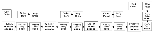
Figure 1: The Initial Setup for the Board Game Version of the Beer Game (taken from Adams et al. 2008) The objective of the game is to fill all customer orders without carrying excessive inventories or having excessive backlogs. The players must fill backlogs eventually. For the first several periods of the game, the customer orders are at four units each period. At some point, the customer orders jump to eight units and remain at that level for the rest of the game. The only stochastic part of the beer game is the human behavior in placing orders but human behavior rarely fails to produce the bullwhip effect. The game runs for 50 periods or until the players become frustrated with excessive backlogs and inventories and the point about the bullwhip effect has been made.
Methodology
The objective of this work is to find whether using information about inventory levels and components of the supply line into an ordering strategy is superior to the JIT pull strategy and the use of POS data at all levels of supply chain. To explore this, cost incurred and profit obtained by each member in a four-echelon supply chain (manufacturer, distributor, wholesaler, and retailer) are computed. For finding the costs incurred and profit obtained, data from spreadsheet beer game simulation developed by Adams et al. (2008) is used. After calculating costs and profit for each player of the supply chain, graphs are plotted between cost versus week (period) and profit versus week for seven different ordering strategies. These graphs have also been plotted for different lead times by Sammidi (2008); however, this paper uses the lead time of two periods.
Sterman (1989) developed an expression for ordering behavior in the beer game in terms of adjustment heuristic that is,
I0t = L̂t + ASt + ASLt
Where:
・I0t – Order rate in time period t,
・L̂t – expected demand in period t,
・ASt – Difference between the desired stock and actual stock in period t, and
・ASLt – Difference between the desired and actual supply line in time period t.
The anchoring heuristic L̂t is often determined using exponential smoothing as follows:
L̂t = θLt-1 + (1-θ)L̂t-1
Where Lt-1 is the demand for the previous period, L̂t-1 is the forecast value of demand for previous period, θ is a parameter varying between 0 and 1.
The adjustment for stock ASt is the difference between the desired stock S* and the actual stock St multiplied by a parameter αs (0 ≤ αs ≤ 1) specifying the fraction of the difference ordered each period.
ASt = αs(S* – St)
The adjustment for supply line is the difference between desired supply line SL* and the actual supply line multiplied by a parameter αSL specifying the fraction of the difference ordered each period.
ASLt = αSL(SL*t – SLt)
The supply line consists of orders in mail delays, the immediately upstream supplier’s backlog, and the material in shipping delays (Adams et al., 2008). We can have for orders: 0 ≤αSLO ≤ 1; for material: 0 ≤ αSLM ≤ 1; and for upstream backlog 0 ≤ αSLB ≤ 1.
The cost incurred by each member is calculated by finding the various costs involved. The cost includes the price of the product, ordering cost, holding costs or inventory cost, and the backlog cost. The backlog cost is the cost, which the supplier must pay as a penalty if he/she cannot deliver the product within the time actually agreed upon. The backlog cost per item is computed by assuming it to be double the cost of the inventory per item (Nienhaus, Zeigenbein, & Schoensleben, 2006). Thus,
Total cost = (Cost per item*number of items ordered) + Ordering cost + Inventory cost (2*Inventory cost per item*number of backlog items)
The ordering cost per order and inventory cost per item are assumed to be $100 and $0.5, respectively for each member in the four-echelon supply chain. Hence,
Total cost = Price per item*number of items ordered + 100 + 0.5*number of items in Inventory + 2*0.5* number of backlog items.
The value of price per item increases from manufacturer to retailer. The price per item for the manufacturer is assumed to be $10, and then it is increased by 2.5 times $10 when it comes to the distributor and then 2.5 times the price of the distributor for the wholesaler and then again 2.5 times the price of the wholesaler for the retailer. Thus, the price per item for distributor is $25, for wholesaler it is $62.5 and for the retailer it is $156.25. The number of items ordered, the number of items in inventory, and the backlogs values have been taken from the simulation developed by Adams et al. (2008). After finding the total cost incurred for each member, the revenue of each member of the supply chain is calculated. The revenue for the manufacturer is the price that the distributor pays for the product; the revenue for the distributor is the price that the wholesaler pays for the product; and the revenue for the wholesaler is the price that the retailer pays for the product.
Profit of each member is calculated by deducting their cost incurred from their revenue obtained, and graphs are developed for seven different cases. Sammidi (2008) contains the detailed work. The seven cases are shown in Table 1.
| Case | L̂t | ASt | ASLt |
|---|---|---|---|
| 1 | θ = 1, (Pull) | αs = 1, (12 – (inv – bklg)) | None |
| 2 | Pull | 12 – (inv – bklg) | αSLO = 1, αSLM = 0, αSLB = 0, (Less orders) |
| 3 | Pull | 12 – (inv – bklg) | αSLO = 0, αSLM = 1, αSLB = 0, (Less material) |
| 4 | Pull | 12 – (inv – bklg) | αSLO = 1, αSLM = 1, αSLB = 0, (Less material and orders) |
| 5 | Pull | 12 – (inv – bklg) | αSLO = 1, αSLM = 1, αSLB = 1, (Less material, orders, and upstream supplier’s backlog) |
| 6 | Pull | αs = 0, None | None |
| 7 | POS | Not applicable | Not applicable |
Among the seven cases mentioned, the first five cases demonstrate the reduction in bullwhip effect as more and more information is interpreted into the supply line. The first case uses an anchoring heuristic of ordering what was ordered, which is equivalent to the pull system, but with a stock adjustment of the full difference between the ideal stock of 12 and the inventory level, that is, 12 – (inventory – backlog). This case displays the largest bullwhip effect as shown in Figures 2-3 of all cases studied. Cases 2 – 5 use the same anchoring and stock adjustment heuristics of Case 1, but they have supply line adjustment heuristics that compensate for more and more of the supply line (orders in mail delays, material in shipping delays, and immediate upstream supplier’s backlog). As more and more of the supply line is compensated, the bullwhip effect diminishes in Cases 2 – 4 until it is completely eliminated in Case 5, when the entire supply line consisting of the sum of the orders in mail delays, the immediate upstream supplier’s backlog, and the material in shipping delays is accounted for.
This paper shows graphs in Figures 2 – 6 for cost and profit versus period (week) for four cases with lead time of two periods. Because profit is revenue minus cost, the profit graph takes into consideration the effect on cost. Hence, there is no need to display the cost versus week graph for each of the cases. Cost and profit for Case 1 are displayed in Figures 2 and 3. Case 1 illustrates the maximum bullwhip effect when no supply chain line information is provided. Case 5 (Figure 4), Case 6 (Figure 5), and Case 7 (Figure 6) show that the bullwhip effect is eliminated. In Case 5, adjustments for supply chain in terms of order delay, material in shipping delay, and upstream backlog have been taken into account. Case 6 is pull strategy, which does not adjust for either stock or supply line. It does not show any bullwhip but produces a steady-state error. This error is better than the bullwhip effect. Also the steady error of Case 6 is slightly better than that of Case 5. In Case 7 there is complete exchange of data between the members of the supply chain, which eliminates the bullwhip effect. However, Case 6 and Case 7 both require discipline and at times are not easy for companies to follow.
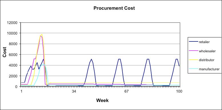
Figure 2. Case 1: Cost for Maximum Bullwhip Effect without Supply Line Informatio
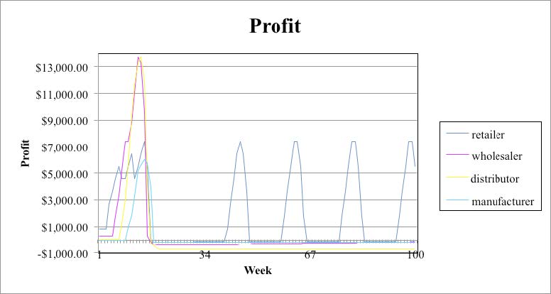
Figure 3. Case 1: Profit for Maximum Bullwhip Effect without Supply Line Information
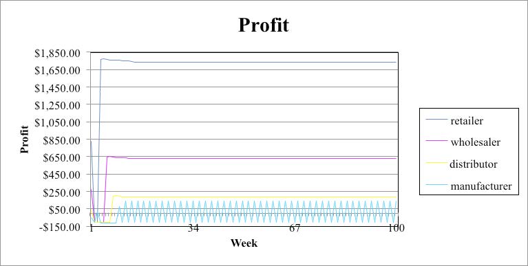
Figure 4. Case 5: Elimination of Bullwhip Effect on Profit by Compensation for Material, Orders, and Upstream Supplier’s Backlog in the Supply Line
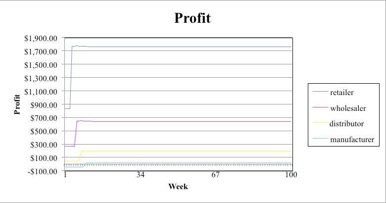
Figure 5. Case 6: Elimination of Bullwhip Effect on Profit by Pull Strategy
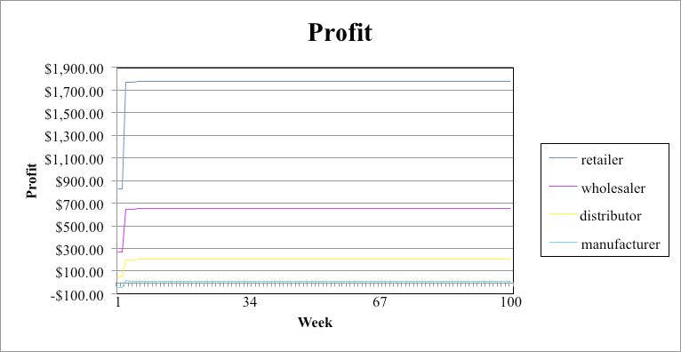
Figure 6. Case 7: POS Eliminates Bullwhip Effect and Backlog
Conclusion
This study is an extension of the work done by Adams et al. (2008), and it uses the beer game spread sheet simulation developed by them. The beer game (Sterman, 1992), shows information and material flow in a four-echelon supply chain. An attempt has been made in the current work to find an ordering strategy that is easy to employ and can minimize the bullwhip effect. Five strategies (Case 1 through Case 5) with different levels of information about inventory and components along the supply line have been compared with the JIT pull strategy (Case 6) and the usage of POS data (Case 7). The cost incurred and profit obtained by each player (manufacturer, distributor, wholesaler, and retailer) of the supply chain for the seven ordering strategies have been determined. Graphs for cost and profit versus time have been plotted.
From the graphs it is evident that as more and more information is provided for the inventory and components along the supply line from Case 1 through Case 5, the bullwhip effect is reduced. Case 1 uses an anchoring heuristic of ordering what was ordered and a stock adjustment to compensate for the difference between the ideal stock and the inventory level. This case shows the largest bullwhip effect. Cases 2 – 5 use the same anchoring and stock adjustment heuristics of Case 1, but have supply line adjustment heuristics that compensate for more and more of the supply line. As more and more of the supply line is compensated, the bullwhip effect diminishes in Cases 2 – 4 until it is completely eliminated in Case 5, when the entire supply line consisting of the sum of the orders in mail delays, the immediate upstream supplier’s backlog, and the material in shipping delays is accounted for.
Case 6 is a pull strategy, which does not adjust for either stock or supply line. It does not show any bullwhip, but it produces a steady-state error. This error is better than the bullwhip effect. Also the steady error of Case 6 is slightly better than that of Case 5. In Case 7 there is complete exchange of data between the members of the supply chain, which eliminates the bullwhip effect. Thus, Case 7 where POS data is used is the best strategy that eliminates the bullwhip effect and Case 6 (pull strategy) is the next best. However, Case 6 and Case 7 both require discipline and at times are not easy for companies to follow. POS has an additional issue because of the reluctance between each member of the supply chain to share information. In such circumstances, Case 5 is a reasonable strategy with better applicability.
Candela Citations
- Reducing the Bullwhip Effect in the Supply Chain: A Study of Different Ordering Strategies. Authored by: M. Affan Badar, Shyamsundarreddy Sammidi, Leslie Gardner. Located at: http://scholar.lib.vt.edu/ejournals/JOTS/v39/v39n1/badar.html. License: CC BY: Attribution