Learning Objectives
By the end of this section, you will be able to:
- Describe the mysteries of atomic spectra.
- Explain Bohr’s theory of the hydrogen atom.
- Explain Bohr’s planetary model of the atom.
- Illustrate energy state using the energy-level diagram.
- Describe the triumphs and limits of Bohr’s theory.
The great Danish physicist Niels Bohr (1885–1962) made immediate use of Rutherford’s planetary model of the atom. (Figure 1). Bohr became convinced of its validity and spent part of 1912 at Rutherford’s laboratory. In 1913, after returning to Copenhagen, he began publishing his theory of the simplest atom, hydrogen, based on the planetary model of the atom. For decades, many questions had been asked about atomic characteristics. From their sizes to their spectra, much was known about atoms, but little had been explained in terms of the laws of physics. Bohr’s theory explained the atomic spectrum of hydrogen and established new and broadly applicable principles in quantum mechanics.
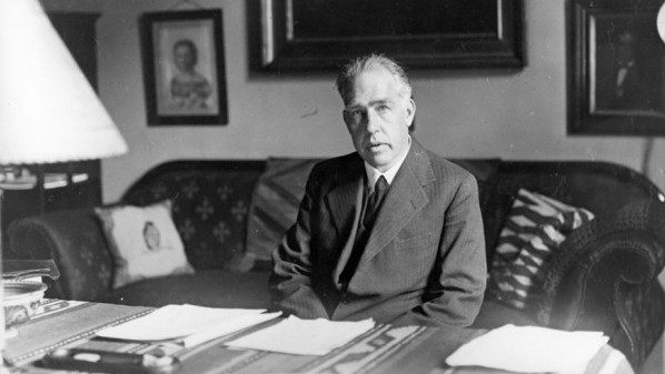
Figure 1. Niels Bohr, Danish physicist, used the planetary model of the atom to explain the atomic spectrum and size of the hydrogen atom. His many contributions to the development of atomic physics and quantum mechanics, his personal influence on many students and colleagues, and his personal integrity, especially in the face of Nazi oppression, earned him a prominent place in history. (credit: Unknown Author, via Wikimedia Commons)
Mysteries of Atomic Spectra
As noted in Quantization of Energy, the energies of some small systems are quantized. Atomic and molecular emission and absorption spectra have been known for over a century to be discrete (or quantized). (See Figure 2.) Maxwell and others had realized that there must be a connection between the spectrum of an atom and its structure, something like the resonant frequencies of musical instruments. But, in spite of years of efforts by many great minds, no one had a workable theory. (It was a running joke that any theory of atomic and molecular spectra could be destroyed by throwing a book of data at it, so complex were the spectra.) Following Einstein’s proposal of photons with quantized energies directly proportional to their wavelengths, it became even more evident that electrons in atoms can exist only in discrete orbits.
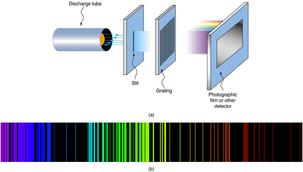
Figure 2. Part (a) shows, from left to right, a discharge tube, slit, and diffraction grating producing a line spectrum. Part (b) shows the emission line spectrum for iron. The discrete lines imply quantized energy states for the atoms that produce them. The line spectrum for each element is unique, providing a powerful and much used analytical tool, and many line spectra were well known for many years before they could be explained with physics. (credit for (b): Yttrium91, Wikimedia Commons)
In some cases, it had been possible to devise formulas that described the emission spectra. As you might expect, the simplest atom—hydrogen, with its single electron—has a relatively simple spectrum. The hydrogen spectrum had been observed in the infrared (IR), visible, and ultraviolet (UV), and several series of spectral lines had been observed. (See Figure 3.) These series are named after early researchers who studied them in particular depth.
The observed hydrogen-spectrum wavelengths can be calculated using the following formula:
[latex]\displaystyle\frac{1}{\lambda}=R\left(\frac{1}{n_{\text{f}}^2}-\frac{1}{n_{\text{i}}^2}\right)\\[/latex],
where λ is the wavelength of the emitted EM radiation and R is the Rydberg constant, determined by the experiment to be R = 1.097 × 10⁷ / m (or m−1).
The constant nf is a positive integer associated with a specific series. For the Lyman series, nf = 1; for the Balmer series, nf = 2; for the Paschen series, nf = 3; and so on. The Lyman series is entirely in the UV, while part of the Balmer series is visible with the remainder UV. The Paschen series and all the rest are entirely IR. There are apparently an unlimited number of series, although they lie progressively farther into the infrared and become difficult to observe as nf increases. The constant ni is a positive integer, but it must be greater than nf. Thus, for the Balmer series, nf = 2 and ni = 3, 4, 5, 6, …. Note that ni can approach infinity. While the formula in the wavelengths equation was just a recipe designed to fit data and was not based on physical principles, it did imply a deeper meaning. Balmer first devised the formula for his series alone, and it was later found to describe all the other series by using different values of nf. Bohr was the first to comprehend the deeper meaning. Again, we see the interplay between experiment and theory in physics. Experimentally, the spectra were well established, an equation was found to fit the experimental data, but the theoretical foundation was missing.
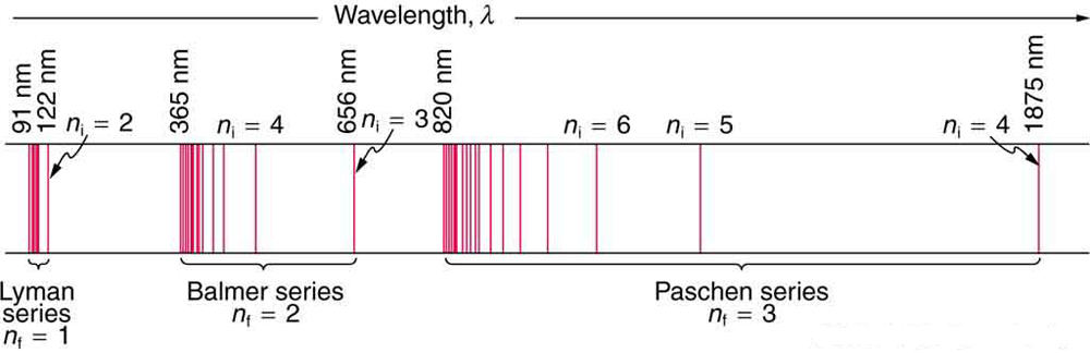
Figure 3. A schematic of the hydrogen spectrum shows several series named for those who contributed most to their determination. Part of the Balmer series is in the visible spectrum, while the Lyman series is entirely in the UV, and the Paschen series and others are in the IR. Values of nf and ni are shown for some of the lines.
Example 1. Calculating Wave Interference of a Hydrogen Line
What is the distance between the slits of a grating that produces a first-order maximum for the second Balmer line at an angle of 15º?
Strategy and Concept
For an Integrated Concept problem, we must first identify the physical principles involved. In this example, we need to know two things:
- the wavelength of light
- the conditions for an interference maximum for the pattern from a double slit
Part 1 deals with a topic of the present chapter, while Part 2 considers the wave interference material of Wave Optics.
Solution for Part 1
Hydrogen spectrum wavelength. The Balmer series requires that nf = 2. The first line in the series is taken to be for ni = 3, and so the second would have ni = 4.
The calculation is a straightforward application of the wavelength equation. Entering the determined values for nf and ni yields
[latex]\begin{array}{lll}\frac{1}{\lambda}&=&R\left(\frac{1}{n_{\text{f}}^2}-\frac{1}{n_{\text{i}}^2}\right)\\\text{ }&=&\left(1.097\times10^7\text{ m}^-1\right)\left(\frac{1}{2^2}-\frac{1}{4^2}\right)\\\text{ }&=&2.057\times10^6\text{ m}^{-1}\end{array}\\[/latex]
Inverting to find λ gives
[latex]\begin{array}{lll}\lambda&=&\frac{1}{2.057\times10^6\text{ m}^-1}=486\times10^{-9}\text{ m}\\\text{ }&=&486\text{ nm}\end{array}\\[/latex]
Discussion for Part 1
This is indeed the experimentally observed wavelength, corresponding to the second (blue-green) line in the Balmer series. More impressive is the fact that the same simple recipe predicts all of the hydrogen spectrum lines, including new ones observed in subsequent experiments. What is nature telling us?
Solution for Part 2
Double-slit interference (Wave Optics). To obtain constructive interference for a double slit, the path length difference from two slits must be an integral multiple of the wavelength. This condition was expressed by the equation d sin θ = mλ, where d is the distance between slits and θ is the angle from the original direction of the beam. The number m is the order of the interference; m=1 in this example. Solving for d and entering known values yields
[latex]\displaystyle{d}=\frac{\left(1\right)\left(486\text{ nm}\right)}{\sin15^{\circ}}=1.88\times10^{-6}\text{ m}\\[/latex]
Discussion for Part 2
This number is similar to those used in the interference examples of Introduction to Quantum Physics (and is close to the spacing between slits in commonly used diffraction glasses).
Bohr’s Solution for Hydrogen
Bohr was able to derive the formula for the hydrogen spectrum using basic physics, the planetary model of the atom, and some very important new proposals. His first proposal is that only certain orbits are allowed: we say that the orbits of electrons in atoms are quantized. Each orbit has a different energy, and electrons can move to a higher orbit by absorbing energy and drop to a lower orbit by emitting energy. If the orbits are quantized, the amount of energy absorbed or emitted is also quantized, producing discrete spectra. Photon absorption and emission are among the primary methods of transferring energy into and out of atoms. The energies of the photons are quantized, and their energy is explained as being equal to the change in energy of the electron when it moves from one orbit to another. In equation form, this is ΔE = hf = Ei − Ef.
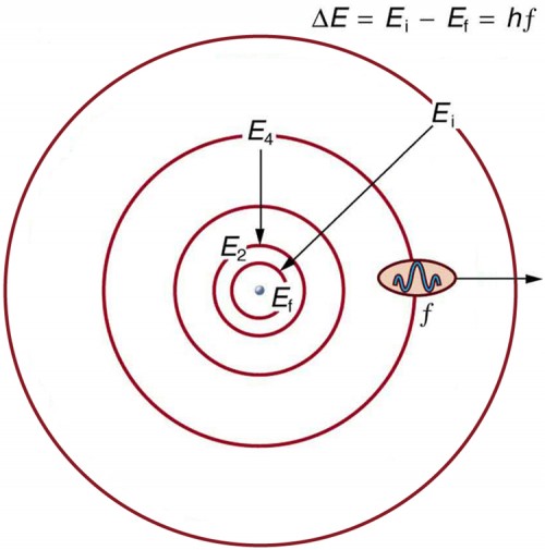
Figure 4. The planetary model of the atom, as modified by Bohr, has the orbits of the electrons quantized. Only certain orbits are allowed, explaining why atomic spectra are discrete (quantized). The energy carried away from an atom by a photon comes from the electron dropping from one allowed orbit to another and is thus quantized. This is likewise true for atomic absorption of photons.
Here, ΔE is the change in energy between the initial and final orbits, and hf is the energy of the absorbed or emitted photon. It is quite logical (that is, expected from our everyday experience) that energy is involved in changing orbits. A blast of energy is required for the space shuttle, for example, to climb to a higher orbit. What is not expected is that atomic orbits should be quantized. This is not observed for satellites or planets, which can have any orbit given the proper energy. (See Figure 4.)
Figure 5 shows an energy-level diagram, a convenient way to display energy states. In the present discussion, we take these to be the allowed energy levels of the electron. Energy is plotted vertically with the lowest or ground state at the bottom and with excited states above. Given the energies of the lines in an atomic spectrum, it is possible (although sometimes very difficult) to determine the energy levels of an atom. Energy-level diagrams are used for many systems, including molecules and nuclei. A theory of the atom or any other system must predict its energies based on the physics of the system.
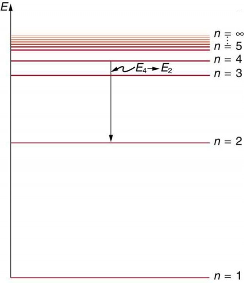
Figure 5. An energy-level diagram plots energy vertically and is useful in visualizing the energy states of a system and the transitions between them. This diagram is for the hydrogen-atom electrons, showing a transition between two orbits having energies E4 and E2.
Bohr was clever enough to find a way to calculate the electron orbital energies in hydrogen. This was an important first step that has been improved upon, but it is well worth repeating here, because it does correctly describe many characteristics of hydrogen. Assuming circular orbits, Bohr proposed that the angular momentum L of an electron in its orbit is quantized, that is, it has only specific, discrete values. The value for L is given by the formula [latex]L=m_{e}vr_{n}=n\frac{h}{2\pi}\left(n=1,2,3,\dots\right)\\[/latex], where L is the angular momentum, me is the electron’s mass, rn is the radius of the n th orbit, and h is Planck’s constant. Note that angular momentum is L = Iω. For a small object at a radius r, I = mr2 and [latex]\omega=\frac{v}{r}\\[/latex], so that [latex]L=\left(mr^2\right)\frac{v}{r}=mvr\\[/latex]. Quantization says that this value of mvr can only be equal to [latex]\frac{h}{2},\frac{2h}{2},\frac{3h}{2}\\[/latex], etc. At the time, Bohr himself did not know why angular momentum should be quantized, but using this assumption he was able to calculate the energies in the hydrogen spectrum, something no one else had done at the time.
From Bohr’s assumptions, we will now derive a number of important properties of the hydrogen atom from the classical physics we have covered in the text. We start by noting the centripetal force causing the electron to follow a circular path is supplied by the Coulomb force. To be more general, we note that this analysis is valid for any single-electron atom. So, if a nucleus has Z protons (Z = 1 for hydrogen, 2 for helium, etc.) and only one electron, that atom is called a hydrogen-like atom. The spectra of hydrogen-like ions are similar to hydrogen, but shifted to higher energy by the greater attractive force between the electron and nucleus. The magnitude of the centripetal force is [latex]\frac{m_{e}v^2}{r_n}\\[/latex], while the Coulomb force is [latex]k\frac{\left(Zq_{e}\right)\left(q_e\right)}{r_n^2}\\[/latex]. The tacit assumption here is that the nucleus is more massive than the stationary electron, and the electron orbits about it. This is consistent with the planetary model of the atom. Equating these,
[latex]k\frac{Zq_{e}^2}{r_n^2}=\frac{m_{e}v^2}{r_n}\text{ (Coulomb = centripetal)}\\[/latex].
Angular momentum quantization is stated in an earlier equation. We solve that equation for v, substitute it into the above, and rearrange the expression to obtain the radius of the orbit. This yields:
[latex]\displaystyle{r}_{n}=\frac{n^2}{Z}a_{\text{B}},\text{ for allowed orbits }\left(n=1,2,3\dots\right)\\[/latex],
where aB is defined to be the Bohr radius, since for the lowest orbit (n = 1) and for hydrogen (Z = 1), r1 = aB. It is left for this chapter’s Problems and Exercises to show that the Bohr radius is
[latex]\displaystyle{a}_{\text{B}}=\frac{h^2}{4\pi^2m_{e}kq_{e}^{2}}=0.529\times10^{-10}\text{ m}\\[/latex].
These last two equations can be used to calculate the radii of the allowed (quantized) electron orbits in any hydrogen-like atom. It is impressive that the formula gives the correct size of hydrogen, which is measured experimentally to be very close to the Bohr radius. The earlier equation also tells us that the orbital radius is proportional to n2, as illustrated in Figure 6.
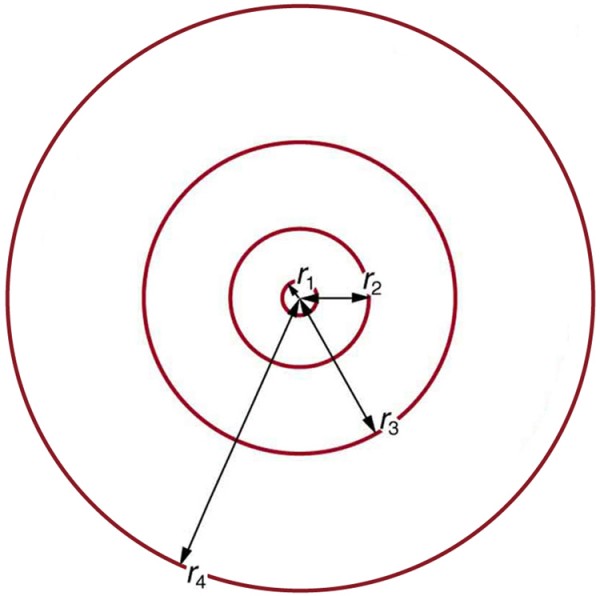
Figure 6. The allowed electron orbits in hydrogen have the radii shown. These radii were first calculated by Bohr and are given by the equation [latex]r_n=\frac{n^2}{Z}a_{\text{B}}\\[/latex]. The lowest orbit has the experimentally verified diameter of a hydrogen atom.
To get the electron orbital energies, we start by noting that the electron energy is the sum of its kinetic and potential energy: En = KE + PE.
Kinetic energy is the familiar [latex]KE=\frac{1}{2}m_{e}v^2\\[/latex], assuming the electron is not moving at relativistic speeds. Potential energy for the electron is electrical, or PE = qeV, where V is the potential due to the nucleus, which looks like a point charge. The nucleus has a positive charge Zqe ; thus, [latex]V=\frac{kZq_e}{r_n}\\[/latex], recalling an earlier equation for the potential due to a point charge. Since the electron’s charge is negative, we see that [latex]PE=-\frac{kZq_e}{r_n}\\[/latex]. Entering the expressions for KE and PE, we find
[latex]\displaystyle{E}_{n}=\frac{1}{2}m_{e}v^2-k\frac{Zq_{e}^{2}}{r_{n}}\\[/latex].
Now we substitute rn and v from earlier equations into the above expression for energy. Algebraic manipulation yields
[latex]\displaystyle{E}_{n}=-\frac{Z^2}{n^2}E_0\left(n=1,2,3,\dots\right)\\[/latex]
for the orbital energies of hydrogen-like atoms. Here, E0 is the ground-state energy (n = 1) for hydrogen (Z = 1) and is given by
[latex]\displaystyle{E}_{0}=\frac{2\pi{q}_{e}^{4}m_{e}k^{2}}{h^2}=13.6\text{ eV}\\[/latex]
Thus, for hydrogen,
[latex]\displaystyle{E}_n=-\frac{13.6\text{ eV}}{n^2}\left(n=1,2,3\dots\right)\\[/latex]
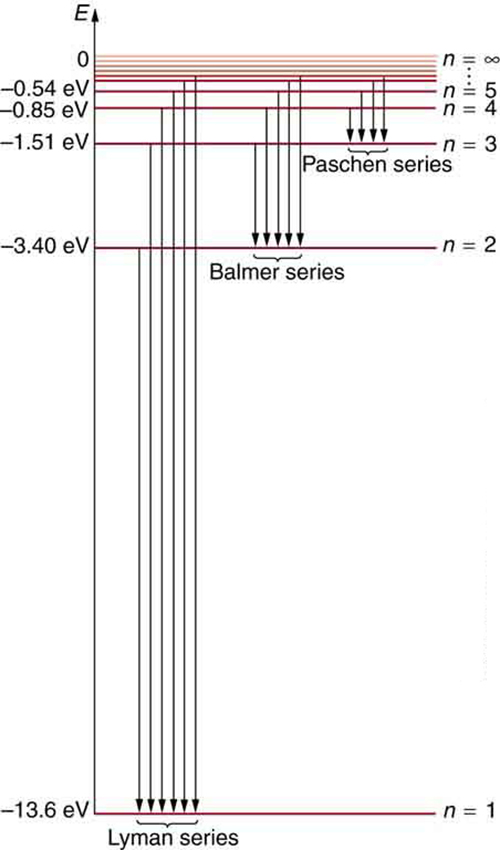
Figure 7. Energy-level diagram for hydrogen showing the Lyman, Balmer, and Paschen series of transitions. The orbital energies are calculated using the above equation, first derived by Bohr.
Figure 7 shows an energy-level diagram for hydrogen that also illustrates how the various spectral series for hydrogen are related to transitions between energy levels.
Electron total energies are negative, since the electron is bound to the nucleus, analogous to being in a hole without enough kinetic energy to escape. As n approaches infinity, the total energy becomes zero. This corresponds to a free electron with no kinetic energy, since rn gets very large for large n, and the electric potential energy thus becomes zero. Thus, 13.6 eV is needed to ionize hydrogen (to go from –13.6 eV to 0, or unbound), an experimentally verified number. Given more energy, the electron becomes unbound with some kinetic energy. For example, giving 15.0 eV to an electron in the ground state of hydrogen strips it from the atom and leaves it with 1.4 eV of kinetic energy.
Finally, let us consider the energy of a photon emitted in a downward transition, given by the equation to be ∆E = hf = Ei − Ef.
Substituting En = (–13.6 eV/n2), we see that
[latex]\displaystyle{hf}=\left(13.6\text{ eV}\right)\left(\frac{1}{n_{\text{f}}^2}-\frac{1}{n_{\text{i}}^2}\right)\\[/latex]
Dividing both sides of this equation by hc gives an expression for [latex]\frac{1}{\lambda}\\[/latex]:
[latex]\displaystyle\frac{hf}{hc}=\frac{f}{c}=\frac{1}{\lambda}=\frac{\left(13.6\text{ eV}\right)}{hc}\left(\frac{1}{n_{\text{f}}^2}-\frac{1}{n_{\text{i}}^2}\right)\\[/latex]
It can be shown that
[latex]\displaystyle\left(\frac{13.6\text{ eV}}{hc}\right)=\frac{\left(13.6\text{ eV}\right)\left(1.602\times10^{-19}\text{ J/eV}\right)}{\left(6.626\times10^{-34}\text{ J }\cdot\text{ s}\right)\left(2.998\times10^{8}\text{ m/s}\right)}=1.097\times10^7\text{ m}^{-1}=R\\[/latex]
is the Rydberg constant. Thus, we have used Bohr’s assumptions to derive the formula first proposed by Balmer years earlier as a recipe to fit experimental data.
[latex]\displaystyle\frac{1}{\lambda}=R\left(\frac{1}{n_{\text{f}}^2}-\frac{1}{n_{\text{i}}^2}\right)\\[/latex]
We see that Bohr’s theory of the hydrogen atom answers the question as to why this previously known formula describes the hydrogen spectrum. It is because the energy levels are proportional to [latex]\frac{1}{n^2}\\[/latex], where n is a non-negative integer. A downward transition releases energy, and so ni must be greater than nf. The various series are those where the transitions end on a certain level. For the Lyman series, nf = 1—that is, all the transitions end in the ground state (see also Figure 7). For the Balmer series, nf = 2, or all the transitions end in the first excited state; and so on. What was once a recipe is now based in physics, and something new is emerging—angular momentum is quantized.
Triumphs and Limits of the Bohr Theory
Bohr did what no one had been able to do before. Not only did he explain the spectrum of hydrogen, he correctly calculated the size of the atom from basic physics. Some of his ideas are broadly applicable. Electron orbital energies are quantized in all atoms and molecules. Angular momentum is quantized. The electrons do not spiral into the nucleus, as expected classically (accelerated charges radiate, so that the electron orbits classically would decay quickly, and the electrons would sit on the nucleus—matter would collapse). These are major triumphs.
But there are limits to Bohr’s theory. It cannot be applied to multielectron atoms, even one as simple as a two-electron helium atom. Bohr’s model is what we call semiclassical. The orbits are quantized (nonclassical) but are assumed to be simple circular paths (classical). As quantum mechanics was developed, it became clear that there are no well-defined orbits; rather, there are clouds of probability. Bohr’s theory also did not explain that some spectral lines are doublets (split into two) when examined closely. We shall examine many of these aspects of quantum mechanics in more detail, but it should be kept in mind that Bohr did not fail. Rather, he made very important steps along the path to greater knowledge and laid the foundation for all of atomic physics that has since evolved.
PhET Explorations: Models of the Hydrogen Atom
How did scientists figure out the structure of atoms without looking at them? Try out different models by shooting light at the atom. Check how the prediction of the model matches the experimental results.
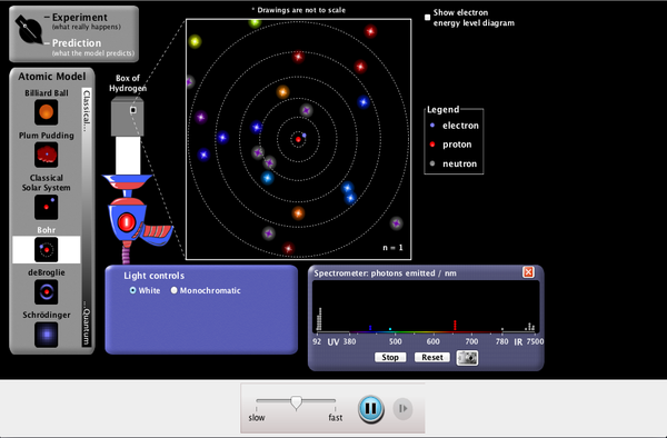
Click to download the simulation. Run using Java.
Section Summary
- The planetary model of the atom pictures electrons orbiting the nucleus in the way that planets orbit the sun. Bohr used the planetary model to develop the first reasonable theory of hydrogen, the simplest atom. Atomic and molecular spectra are quantized, with hydrogen spectrum wavelengths given by the formula
[latex]\frac{1}{\lambda }=R\left(\frac{1}{{n}_{\text{f}}^{2}}-\frac{1}{{n}_{\text{i}}^{2}}\right)\\[/latex],
where λ is the wavelength of the emitted EM radiation and R is the Rydberg constant, which has the value R = 1.097 × 10⁷ m−1. - The constants ni and nf are positive integers, and ni must be greater than nf.
- Bohr correctly proposed that the energy and radii of the orbits of electrons in atoms are quantized, with energy for transitions between orbits given by ∆E = hf = Ei − Ef, where ∆E is the change in energy between the initial and final orbits and hf is the energy of an absorbed or emitted photon. It is useful to plot orbital energies on a vertical graph called an energy-level diagram.
- Bohr proposed that the allowed orbits are circular and must have quantized orbital angular momentum given by [latex]L={m}_{e}{\text{vr}}_{n}=n\frac{h}{2\pi }\left(n=1, 2, 3 \dots \right)\\[/latex], where L is the angular momentum, rn is the radius of the nth orbit, and h is Planck’s constant. For all one-electron (hydrogen-like) atoms, the radius of an orbit is given by [latex]{r}_{n}=\frac{{n}^{2}}{Z}{a}_{\text{B}}\left(\text{allowed orbits }n=1, 2, 3, ...\right)\\[/latex], Z is the atomic number of an element (the number of electrons is has when neutral) and aB is defined to be the Bohr radius, which is [latex]{a}_{\text{B}}=\frac{{h}^{2}}{{4\pi }^{2}{m}_{e}{\text{kq}}_{e}^{2}}=\text{0.529}\times {\text{10}}^{-\text{10}}\text{ m}\\[/latex].
- Furthermore, the energies of hydrogen-like atoms are given by [latex]{E}_{n}=-\frac{{Z}^{2}}{{n}^{2}}{E}_{0}\left(n=1, 2, 3 ...\right)\\[/latex], where E0 is the ground-state energy and is given by [latex]{E}_{0}=\frac{{2\pi }^{2}{q}_{e}^{4}{m}_{e}{k}^{2}}{{h}^{2}}=\text{13.6 eV}\\[/latex].
Thus, for hydrogen, [latex]{E}_{n}=-\frac{\text{13.6 eV}}{{n}^{2}}\left(n,=,1, 2, 3 ...\right)\\[/latex]. - The Bohr Theory gives accurate values for the energy levels in hydrogen-like atoms, but it has been improved upon in several respects.
Conceptual Questions
- How do the allowed orbits for electrons in atoms differ from the allowed orbits for planets around the sun? Explain how the correspondence principle applies here.
- Explain how Bohr’s rule for the quantization of electron orbital angular momentum differs from the actual rule.
- What is a hydrogen-like atom, and how are the energies and radii of its electron orbits related to those in hydrogen?
Problems & Exercises
- By calculating its wavelength, show that the first line in the Lyman series is UV radiation.
- Find the wavelength of the third line in the Lyman series, and identify the type of EM radiation.
- Look up the values of the quantities in [latex]{a}_{\text{B}}=\frac{{h}^{2}}{{4\pi }^{2}{m}_{e}{\text{kq}}_{e}^{2}}\\[/latex] , and verify that the Bohr radius aB is 0.529 × 10⁻¹⁰ m.
- Verify that the ground state energy E0 is 13.6 eV by using [latex]{E}_{0}=\frac{{2\pi }^{2}{q}_{e}^{4}{m}_{e}{k}^{2}}{{h}^{2}}\\[/latex].
- If a hydrogen atom has its electron in the n = 4 state, how much energy in eV is needed to ionize it?
- A hydrogen atom in an excited state can be ionized with less energy than when it is in its ground state. What is n for a hydrogen atom if 0.850 eV of energy can ionize it?
- Find the radius of a hydrogen atom in the n = 2 state according to Bohr’s theory.
- Show that [latex]\frac{\left(13.6 \text{eV}\right)}{hc}=1.097\times10^{7}\text{ m}=R\\[/latex] (Rydberg’s constant), as discussed in the text.
- What is the smallest-wavelength line in the Balmer series? Is it in the visible part of the spectrum?
- Show that the entire Paschen series is in the infrared part of the spectrum. To do this, you only need to calculate the shortest wavelength in the series.
- Do the Balmer and Lyman series overlap? To answer this, calculate the shortest-wavelength Balmer line and the longest-wavelength Lyman line.
- (a) Which line in the Balmer series is the first one in the UV part of the spectrum? (b) How many Balmer series lines are in the visible part of the spectrum? (c) How many are in the UV?
- A wavelength of 4.653 µm is observed in a hydrogen spectrum for a transition that ends in the nf = 5 level. What was ni for the initial level of the electron?
- A singly ionized helium ion has only one electron and is denoted He+. What is the ion’s radius in the ground state compared to the Bohr radius of hydrogen atom?
- A beryllium ion with a single electron (denoted Be3+) is in an excited state with radius the same as that of the ground state of hydrogen. (a) What is n for the Be3+ ion? (b) How much energy in eV is needed to ionize the ion from this excited state?
- Atoms can be ionized by thermal collisions, such as at the high temperatures found in the solar corona. One such ion is C+5, a carbon atom with only a single electron. (a) By what factor are the energies of its hydrogen-like levels greater than those of hydrogen? (b) What is the wavelength of the first line in this ion’s Paschen series? (c) What type of EM radiation is this?
- Verify Equations [latex]{r}_{n}=\frac{{n}^{2}}{Z}{a}_{\text{B}}\\[/latex] and [latex]{a}_{B}=\frac{{h}^{2}}{{4\pi }^{2}{m}_{e}{kq}_{e}^{2}}=0.529\times{10}^{-10}\text{ m}\\[/latex] using the approach stated in the text. That is, equate the Coulomb and centripetal forces and then insert an expression for velocity from the condition for angular momentum quantization.
- The wavelength of the four Balmer series lines for hydrogen are found to be 410.3, 434.2, 486.3, and 656.5 nm. What average percentage difference is found between these wavelength numbers and those predicted by [latex]\frac{1}{\lambda}=R\left(\frac{1}{{n}_{\text{f}}^{2}}-\frac{1}{{n}_{\text{i}}^{2}}\right)\\[/latex]? It is amazing how well a simple formula (disconnected originally from theory) could duplicate this phenomenon.
Glossary
hydrogen spectrum wavelengths: the wavelengths of visible light from hydrogen; can be calculated by
[latex]\displaystyle\frac{1}{\lambda }=R\left(\frac{1}{{n}_{\text{f}}^{2}}-\frac{1}{{n}_{\text{i}}^{2}}\right)\\[/latex]
Rydberg constant: a physical constant related to the atomic spectra with an established value of 1.097 × 10⁷ m−1
double-slit interference: an experiment in which waves or particles from a single source impinge upon two slits so that the resulting interference pattern may be observed
energy-level diagram: a diagram used to analyze the energy level of electrons in the orbits of an atom
Bohr radius: the mean radius of the orbit of an electron around the nucleus of a hydrogen atom in its ground state
hydrogen-like atom: any atom with only a single electron
energies of hydrogen-like atoms: Bohr formula for energies of electron states in hydrogen-like atoms: [latex]{E}_{n}=-\frac{{Z}^{2}}{{n}^{2}}{E}_{0}\left(n=\text{1, 2, 3,}\dots \right)\\[/latex]
Selected Solutions to Problems & Exercises
1. [latex]\displaystyle\frac{1}{\lambda}=R\left(\frac{1}{{n}_{\text{f}}^{2}}-\frac{1}{{n}_{\text{i}}^{2}}\right)\Rightarrow \lambda =\frac{1}{R}\left[\frac{\left({n}_{\text{i}}\cdot{n}_{\text{f}}\right)^{2}}{{n}_{\text{i}}^{2}-{n}_{\text{f}}^{2}}\right];{n}_{\text{i}}=2,{n}_{\text{f}}=1\\[/latex], so that
[latex]\displaystyle\lambda =\left(\frac{m}{1.097\times {\text{10}}^{7}}\right)\left[\frac{\left(2\times1\right)^{2}}{{2}^{2}-{1}^{2}}\right]=1\text{.}\text{22}\times {\text{10}}^{-7}\text{m}=\text{122 nm}\\[/latex] , which is UV radiation.
3. [latex]\begin{array}{lll}{a}_{\text{B}}&=&\frac{{h}^{2}}{{4\pi }^{2}{m}_{e}{\text{kZq}}_{e}^{2}}\\\text{ }&=&\frac{\left(\text{6.626}\times {\text{10}}^{-\text{34}}\text{J }\cdot\text{ s}\right)^{2}}{{4\pi }^{2}\left(9.109\times {\text{10}}^{-\text{31}}\text{kg}\right)\left(8.988\times {\text{10}}^{9}\text{N}\cdot{\text{m}}^{2}/{C}^{2}\right)\left(1\right)\left(1.602\times {\text{10}}^{-\text{19}}\text{C}\right)^{2}}\\\text{ }&=&\text{0.529}\times {\text{10}}^{-\text{10}}\text{m}\end{array}\\[/latex]
5. 0.850 eV
7. 2.12 × 10⁻¹⁰ m
9. 365 nm; it is in the ultraviolet.
11. No overlap; 365 nm; 122 nm
13. 7
15. (a) 2; (b) 54.4 eV
17. [latex]\displaystyle\frac{{\text{kZq}}_{e}^{2}}{{r}_{n}^{2}}=\frac{{m}_{e}{V}^{2}}{{r}_{n}}\\[/latex], so that [latex]\displaystyle{r}_{n}=\frac{{\text{kZq}}_{e}^{2}}{{m}_{e}{V}^{2}}=\frac{{\text{kZq}}_{e}^{2}}{{m}_{e}}\frac{1}{{V}^{2}}\\[/latex]. From the equation [latex]\displaystyle{m}_{e}{vr}_{n}=n\frac{h}{2\pi}\\[/latex], we can substitute for the velocity, giving:
[latex]\displaystyle{r}_{n}=\frac{{\text{kZq}}_{e}^{2}}{{m}_{e}}\cdot \frac{{4\pi }^{2}{m}_{e}^{2}{r}_{n}^{2}}{{n}^{2}{h}^{2}}\\[/latex]
so that
[latex]\displaystyle{r}_{n}=\frac{{n}^{2}}{Z}\frac{{h}^{2}}{{4\pi }^{2}{m}_{e}{\text{kq}}_{e}^{2}}=\frac{{n}^{2}}{Z}{a}_{\text{B}}\\[/latex],
where
[latex]\displaystyle{a}_{\text{B}}=\frac{{h}^{2}}{{4\pi }^{2}{m}_{e}{\text{kq}}_{e}^{2}}\\[/latex].
Candela Citations
- College Physics. Authored by: OpenStax College. Located at: http://cnx.org/contents/031da8d3-b525-429c-80cf-6c8ed997733a/College_Physics. License: CC BY: Attribution. License Terms: Located at License
- PhET Interactive Simulations . Provided by: University of Colorado Boulder . Located at: http://phet.colorado.edu. License: CC BY: Attribution