Learning Objectives
- Composite and InverseFunctions
- Define a composite function
- Define an inverse function
- Use compositions of functions to verify inverses algebraically
- Identify an inverse algebraically
- Identify the domain and range of inverse functions with tables
- Logarithmic Functions
- Define a logarithmic function as the inverse of an exponential function
- Convert between logarithmic and exponential forms
- Evaluate Logarithms
- Mentally evaluate logarithms
- Define natural logarithm, evaluate natural logarithms with a calculator
- Define common logarithm, evaluate common logarithms mentally and with a calculator
- Graphs of Logarithmic Functions
- Identify the domain of a logarithmic function.
- Graph logarithmic functions.

Figure 1. Devastation of March 11, 2011 earthquake in Honshu, Japan. (credit: Daniel Pierce)
In 2010, a major earthquake struck Haiti, destroying or damaging over 285,000 homes.[1] One year later, another, stronger earthquake devastated Honshu, Japan, destroying or damaging over 332,000 buildings,[2] like those shown in the picture above. Even though both caused substantial damage, the earthquake in 2011 was 100 times stronger than the earthquake in Haiti. How do we know? The magnitudes of earthquakes are measured on a scale known as the Richter Scale. The Haitian earthquake registered a 7.0 on the Richter Scale[3] whereas the Japanese earthquake registered a 9.0.[4]
The Richter Scale is a base-ten logarithmic scale. In other words, an earthquake of magnitude 8 is not twice as great as an earthquake of magnitude 4. It is [latex]{10}^{8 - 4}={10}^{4}=10,000[/latex] times as great! In this lesson, we will investigate the nature of the Richter Scale and the base-ten function upon which it depends.
Our first topic will be about inverse functions, logarithmic functions are the inverse of an exponential functions, and sometimes understanding this helps us make sense of what a logarithm is.
Composite and Inverse Functions
Suppose we want to calculate how much it costs to heat a house on a particular day of the year. The cost to heat a house will depend on the average daily temperature, and in turn, the average daily temperature depends on the particular day of the year. Notice how we have just defined two relationships: The cost depends on the temperature, and the temperature depends on the day.

Figure 1
Using descriptive variables, we can notate these two functions. The function [latex]C\left(T\right)[/latex] gives the cost [latex]C[/latex] of heating a house for a given average daily temperature in [latex]T[/latex] degrees Celsius. The function [latex]T\left(d\right)[/latex] gives the average daily temperature on day [latex]d[/latex] of the year. For any given day, [latex]\text{Cost}=C\left(T\left(d\right)\right)[/latex] means that the cost depends on the temperature, which in turns depends on the day of the year. Thus, we can evaluate the cost function at the temperature [latex]T\left(d\right)[/latex]. For example, we could evaluate [latex]T\left(5\right)[/latex] to determine the average daily temperature on the 5th day of the year. Then, we could evaluate the cost function at that temperature. We would write [latex]C\left(T\left(5\right)\right)[/latex]. By combining these two relationships into one function, we have performed function composition.
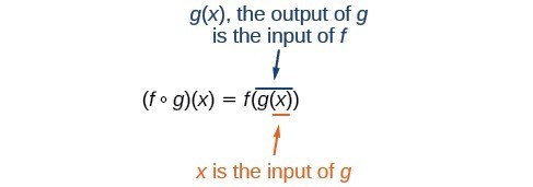
We read the left-hand side as [latex]"f[/latex] composed with [latex]g[/latex] at [latex]x,"[/latex] and the right-hand side as [latex]"f[/latex] of [latex]g[/latex] of [latex]x."[/latex] The two sides of the equation have the same mathematical meaning and are equal. The open circle symbol [latex]\circ[/latex] is called the composition operator.
It is also important to understand the order of operations in evaluating a composite function. We follow the usual convention with parentheses by starting with the innermost parentheses first, and then working to the outside.
Example
Using the functions provided, find [latex]f\left(g\left(x\right)\right)[/latex] and [latex]g\left(f\left(x\right)\right)[/latex].
[latex]f\left(x\right)=2x+1[/latex]
[latex]g\left(x\right)=3-x[/latex]
In the following video you will see another example of how to find the composition of two functions.
Inverse Functions
An inverse function is a function for which the input of the original function becomes the output of the inverse function. This naturally leads to the output of the original function becoming the input of the inverse function. The reason we want to introduce inverse functions is because exponential and logarithmic functions are inverses of each other, and understanding this quality helps to make understanding logarithmic functions easier. And the reason we introduced composite functions is because you can verify, algebraically, whether two functions are inverses of each other by using a composition.
Given a function [latex]f\left(x\right)[/latex], we represent its inverse as [latex]{f}^{-1}\left(x\right)[/latex], read as [latex]"f[/latex] inverse of [latex]x.\text{"}[/latex] The raised [latex]-1[/latex] is part of the notation. It is not an exponent; it does not imply a power of [latex]-1[/latex] . In other words, [latex]{f}^{-1}\left(x\right)[/latex] does not mean [latex]\frac{1}{f\left(x\right)}[/latex] because [latex]\frac{1}{f\left(x\right)}[/latex] is the reciprocal of [latex]f[/latex] and not the inverse.
Just as zero does not have a reciprocal, some functions do not have inverses.
Inverse Function
For any one-to-one function [latex]f\left(x\right)=y[/latex], a function [latex]{f}^{-1}\left(x\right)[/latex] is an inverse function of [latex]f[/latex] if [latex]{f}^{-1}\left(y\right)=x[/latex].
The notation [latex]{f}^{-1}[/latex] is read [latex]\text{"}f[/latex] inverse.” Like any other function, we can use any variable name as the input for [latex]{f}^{-1}[/latex], so we will often write [latex]{f}^{-1}\left(x\right)[/latex], which we read as [latex]"f[/latex] inverse of [latex]x."[/latex]
Keep in mind that
and not all functions have inverses.
In our first example we will identify an inverse function from ordered pairs.
Example
If for a particular one-to-one function [latex]f\left(2\right)=4[/latex] and [latex]f\left(5\right)=12[/latex], what are the corresponding input and output values for the inverse function?
Analysis of the Solution
In the following video we show an example of finding corresponding input and output values given two ordered pairs from functions that are inverses.
How To: Given two functions [latex]f\left(x\right)[/latex] and [latex]g\left(x\right)[/latex], test whether the functions are inverses of each other.
- Substitute [latex]g(x)[/latex] into [latex]f(x)[/latex]. The result must be x. [latex]f\left(g(x)\right)=x[/latex]
- Substitute [latex]f(x)[/latex] into [latex]g(x)[/latex]. The result must be x. [latex]g\left(f(x)\right)=x[/latex]
If [latex]f(x)[/latex] and [latex]g(x)[/latex] are inverses, then [latex]f(x)=g^{-1}(x)[/latex] and [latex]g(x)=f^{-1}(x)[/latex]
In our next example we will test inverse relationships algebraically.
Example
If [latex]f\left(x\right)=x^2-3[/latex], for [latex]x\ge0[/latex] and [latex]g\left(x\right)=\sqrt{x+3}[/latex], is g the inverse of f? [latex]g={f}^{-1}?[/latex]
In the following video we use algebra to determine if two functions are inverses.
We will show one more example of how to verify whether you have an inverse algebraically.
Example
If [latex]f\left(x\right)=\frac{1}{x+2}[/latex] and [latex]g\left(x\right)=\frac{1}{x}-2[/latex], is g the inverse of f? [latex]g={f}^{-1}?[/latex]
We will show one more example of how to use algebra to determine whether two functions are inverses of each other.
Domain and Range of a Function and It’s Inverse
The outputs of the function [latex]f[/latex] are the inputs to [latex]{f}^{-1}[/latex], so the range of [latex]f[/latex] is also the domain of [latex]{f}^{-1}[/latex]. Likewise, because the inputs to [latex]f[/latex] are the outputs of [latex]{f}^{-1}[/latex], the domain of [latex]f[/latex] is the range of [latex]{f}^{-1}[/latex]. We can visualize the situation.

Domain and range of a function and its inverse
In many cases, if a function is not one-to-one, we can still restrict the function to a part of its domain on which it is one-to-one. For example, we can make a restricted version of the square function [latex]f\left(x\right)={x}^{2}[/latex] with its range limited to [latex]\left[0,\infty \right)[/latex], which is a one-to-one function (it passes the horizontal line test) and which has an inverse (the square-root function).
Domain and Range of Inverse Functions
The range of a function [latex]f\left(x\right)[/latex] is the domain of the inverse function [latex]{f}^{-1}\left(x\right)[/latex].
The domain of [latex]f\left(x\right)[/latex] is the range of [latex]{f}^{-1}\left(x\right)[/latex].
In our last example we will define the domain and range of a function’s inverse using a table of values, and evaluate the inverse at a specific value.
Example
A function [latex]f\left(t\right)[/latex] is given below, showing distance in miles that a car has traveled in [latex]t[/latex] minutes.
- Define the domain and range of the function and it’s inverse.
- Find and interpret [latex]{f}^{-1}\left(70\right)[/latex].
| [latex]t\text{ (minutes)}[/latex] | 30 | 50 | 70 | 90 |
| [latex]f\left(t\right)\text{ (miles)}[/latex] | 20 | 40 | 60 | 70 |
Define Logarithmic Functions
In order to analyze the magnitude of earthquakes or compare the magnitudes of two different earthquakes, we need to be able to convert between logarithmic and exponential form. For example, suppose the amount of energy released from one earthquake were 500 times greater than the amount of energy released from another. We want to calculate the difference in magnitude. The equation that represents this problem is [latex]{10}^{x}=500[/latex], where x represents the difference in magnitudes on the Richter Scale. How would we solve for x?
We have not yet learned a method for solving exponential equations. None of the algebraic tools discussed so far is sufficient to solve [latex]{10}^{x}=500[/latex]. We know that [latex]{10}^{2}=100[/latex] and [latex]{10}^{3}=1000[/latex], so it is clear that x must be some value between 2 and 3, since [latex]y={10}^{x}[/latex] is increasing. We can examine a graph to better estimate the solution.
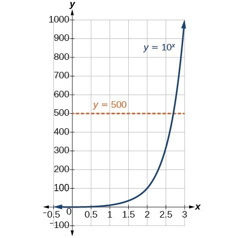
Figure 2
Estimating from a graph, however, is imprecise. To find an algebraic solution, we must introduce a new function. Observe that the graph above passes the horizontal line test. The exponential function [latex]y={b}^{x}[/latex] is one-to-one, so its inverse, [latex]x={b}^{y}[/latex] is also a function. As is the case with all inverse functions, we simply interchange x and y and solve for y to find the inverse function. To represent y as a function of x, we use a logarithmic function of the form [latex]y={\mathrm{log}}_{b}\left(x\right)[/latex]. The base b logarithm of a number is the exponent by which we must raise b to get that number.
We read a logarithmic expression as, “The logarithm with base b of x is equal to y,” or, simplified, “log base b of x is y.” We can also say, “b raised to the power of y is x,” because logs are exponents. For example, the base 2 logarithm of 32 is 5, because 5 is the exponent we must apply to 2 to get 32. Since [latex]{2}^{5}=32[/latex], we can write [latex]{\mathrm{log}}_{2}32=5[/latex]. We read this as “log base 2 of 32 is 5.”
We can express the relationship between logarithmic form and its corresponding exponential form as follows:
Note that the base b is always positive.

Because logarithm is a function, it is most correctly written as [latex]{\mathrm{log}}_{b}\left(x\right)[/latex], using parentheses to denote function evaluation, just as we would with [latex]f\left(x\right)[/latex]. However, when the input is a single variable or number, it is common to see the parentheses dropped and the expression written without parentheses, as [latex]{\mathrm{log}}_{b}x[/latex]. Note that many calculators require parentheses around the x.
We can illustrate the notation of logarithms as follows:

Notice that, comparing the logarithm function and the exponential function, the input and the output are switched. This means [latex]y={\mathrm{log}}_{b}\left(x\right)[/latex] and [latex]y={b}^{x}[/latex] are inverse functions.
Definition of the Logarithmic Function
A logarithm base b of a positive number x satisfies the following definition.
For [latex]x>0,b>0,b\ne 1[/latex],
where,
- we read [latex]{\mathrm{log}}_{b}\left(x\right)[/latex] as, “the logarithm with base b of x” or the “log base b of x.”
- the logarithm y is the exponent to which b must be raised to get x.
Also, since the logarithmic and exponential functions switch the x and y values, the domain and range of the exponential function are interchanged for the logarithmic function. Therefore,
- the domain of the logarithm function with base [latex]b \text{ is} \left(0,\infty \right)[/latex].
- the range of the logarithm function with base [latex]b \text{ is} \left(-\infty ,\infty \right)[/latex].
In our first example we will convert logarithmic equations into exponential equations.
Example
Write the following logarithmic equations in exponential form.
- [latex]{\mathrm{log}}_{6}\left(\sqrt{6}\right)=\frac{1}{2}[/latex]
- [latex]{\mathrm{log}}_{3}\left(9\right)=2[/latex]
Show Answer
In the following video we present more examples of rewriting logarithmic equations as exponential equations.
How To: Given an equation in logarithmic form [latex]{\mathrm{log}}_{b}\left(x\right)=y[/latex], convert it to exponential form.
- Examine the equation [latex]y={\mathrm{log}}_{b}x[/latex] and identify b, y, and x.
- Rewrite [latex]{\mathrm{log}}_{b}x=y[/latex] as [latex]{b}^{y}=x[/latex].
Think About It
Can we take the logarithm of a negative number? Re-read the definition of a logarithm and formulate an answer. Think about the behavior of exponents. You can use the textbox below to formulate your ideas before you look at an answer.
Convert from exponential to logarithmic form
To convert from exponents to logarithms, we follow the same steps in reverse. We identify the base b, exponent x, and output y. Then we write [latex]x={\mathrm{log}}_{b}\left(y\right)[/latex].
Example
Write the following exponential equations in logarithmic form.
- [latex]{2}^{3}=8[/latex]
- [latex]{5}^{2}=25[/latex]
- [latex]{10}^{-4}=\frac{1}{10,000}[/latex]
Show Answer
In our last video we show more examples of writing logarithmic equations as exponential equations.
Evaluate Logarithms
Knowing the squares, cubes, and roots of numbers allows us to evaluate many logarithms mentally. For example, consider [latex]{\mathrm{log}}_{2}8[/latex]. We ask, “To what exponent must 2 be raised in order to get 8?” Because we already know [latex]{2}^{3}=8[/latex], it follows that [latex]{\mathrm{log}}_{2}8=3[/latex].
Now consider solving [latex]{\mathrm{log}}_{7}49[/latex] and [latex]{\mathrm{log}}_{3}27[/latex] mentally.
- We ask, “To what exponent must 7 be raised in order to get 49?” We know [latex]{7}^{2}=49[/latex]. Therefore, [latex]{\mathrm{log}}_{7}49=2[/latex]
- We ask, “To what exponent must 3 be raised in order to get 27?” We know [latex]{3}^{3}=27[/latex]. Therefore, [latex]{\mathrm{log}}_{3}27=3[/latex]
Even some seemingly more complicated logarithms can be evaluated without a calculator. For example, let’s evaluate [latex]{\mathrm{log}}_{\frac{2}{3}}\frac{4}{9}[/latex] mentally.
- We ask, “To what exponent must [latex]\frac{2}{3}[/latex] be raised in order to get [latex]\frac{4}{9}[/latex]? ” We know [latex]{2}^{2}=4[/latex] and [latex]{3}^{2}=9[/latex], so [latex]{\left(\frac{2}{3}\right)}^{2}=\frac{4}{9}[/latex]. Therefore, [latex]{\mathrm{log}}_{\frac{2}{3}}\left(\frac{4}{9}\right)=2[/latex].
In our first example we will evaluate logarithms mentally.
Example
Solve [latex]y={\mathrm{log}}_{4}\left(64\right)[/latex] without using a calculator.
In our first video we will show more examples of evaluating logarithms mentally, this helps you get familiar with what a logarithm represents.
In our next example we will evaluate the logarithm of a reciprocal.
Example
Evaluate [latex]y={\mathrm{log}}_{3}\left(\frac{1}{27}\right)[/latex] without using a calculator.
How To: Given a logarithm of the form [latex]y={\mathrm{log}}_{b}\left(x\right)[/latex], evaluate it mentally.
- Rewrite the argument x as a power of b: [latex]{b}^{y}=x[/latex].
- Use previous knowledge of powers of b identify y by asking, “To what exponent should b be raised in order to get x?”
Natural logarithms
The most frequently used base for logarithms is e. Base e logarithms are important in calculus and some scientific applications; they are called natural logarithms. The base e logarithm, [latex]{\mathrm{log}}_{e}\left(x\right)[/latex], has its own notation, [latex]\mathrm{ln}\left(x\right)[/latex].
Most values of [latex]\mathrm{ln}\left(x\right)[/latex] can be found only using a calculator. The major exception is that, because the logarithm of 1 is always 0 in any base, [latex]\mathrm{ln}1=0[/latex]. For other natural logarithms, we can use the [latex]\mathrm{ln}[/latex] key that can be found on most scientific calculators. We can also find the natural logarithm of any power of e using the inverse property of logarithms.
A General Note: Definition of the Natural Logarithm
A natural logarithm is a logarithm with base e. We write [latex]{\mathrm{log}}_{e}\left(x\right)[/latex] simply as [latex]\mathrm{ln}\left(x\right)[/latex]. The natural logarithm of a positive number x satisfies the following definition.
For [latex]x>0[/latex],
We read [latex]\mathrm{ln}\left(x\right)[/latex] as, “the logarithm with base e of x” or “the natural logarithm of x.”
The logarithm y is the exponent to which e must be raised to get x.
Since the functions [latex]y=e{}^{x}[/latex] and [latex]y=\mathrm{ln}\left(x\right)[/latex] are inverse functions, [latex]\mathrm{ln}\left({e}^{x}\right)=x[/latex] for all x and [latex]e{}^{\mathrm{ln}\left(x\right)}=x[/latex] for x > 0.
In the next example, we will evaluate a natural logarithm using a calculator.
Example
Evaluate [latex]y=\mathrm{ln}\left(500\right)[/latex] to four decimal places using a calculator.
In our next video, we show more examples of how to evaluate natural logarithms using a calculator.
Common logarithms
Sometimes we may see a logarithm written without a base. In this case, we assume that the base is 10. In other words, the expression [latex]{\mathrm{log}}_{}[/latex] means [latex]{\mathrm{log}}_{10}[/latex] We call a base-10 logarithm a common logarithm. Common logarithms are used to measure the Richter Scale mentioned at the beginning of the section. Scales for measuring the brightness of stars and the pH of acids and bases also use common logarithms.
Definition of Common Logarithm: Log is an exponent
A common logarithm is a logarithm with base 10. We write [latex]{\mathrm{log}}_{10}(x)[/latex] simpliy as [latex]{\mathrm{log}}_{}(x)[/latex]. The common logarithm of a positive number, x, satisfies the following definition:
For [latex]x\gt0[/latex]
[latex]y={\mathrm{log}}_{}(x)[/latex] is equivalent to [latex]10^y=x[/latex]
We read [latex]{\mathrm{log}}_{}(x)[/latex] as ” the logarithm with base 10 of x” or “log base 10 of x”.
The logarithm y is the exponent to which 10 must be raised to get x.
Example
Evaluate [latex]{\mathrm{log}}_{}(1000)[/latex] without using a calculator.
Example
Evaluate [latex]y={\mathrm{log}}_{}(321)[/latex] to four decimal places using a calculator.
In our last example we will use a logarithm to find the difference in magnitude of two different earthquakes.
Example
The amount of energy released from one earthquake was 500 times greater than the amount of energy released from another. The equation [latex]10^x=500[/latex] represents this situation, where x is the difference in magnitudes on the Richter Scale. To the nearest thousandth, what was the difference in magnitudes?
Graphs of Logarithmic Functions
Before working with graphs, we will take a look at the domain (the set of input values) for which the logarithmic function is defined.
Recall that the exponential function is defined as [latex]y={b}^{x}[/latex] for any real number x and constant [latex]b>0[/latex], [latex]b\ne 1[/latex], where
- The domain of y is [latex]\left(-\infty ,\infty \right)[/latex].
- The range of y is [latex]\left(0,\infty \right)[/latex].
In the last section we learned that the logarithmic function [latex]y={\mathrm{log}}_{b}\left(x\right)[/latex] is the inverse of the exponential function [latex]y={b}^{x}[/latex]. So, as inverse functions:
- The domain of [latex]y={\mathrm{log}}_{b}\left(x\right)[/latex] is the range of [latex]y={b}^{x}[/latex]:[latex]\left(0,\infty \right)[/latex].
- The range of [latex]y={\mathrm{log}}_{b}\left(x\right)[/latex] is the domain of [latex]y={b}^{x}[/latex]: [latex]\left(-\infty ,\infty \right)[/latex].
How To: Given a logarithmic function, identify the domain.
- Set up an inequality showing the argument greater than zero.
- Solve for x.
- Write the domain in interval notation.
In our first example we will show how to identify the domain of a logarithmic function.
Example
What is the domain of [latex]f\left(x\right)={\mathrm{log}}_{2}\left(x+3\right)[/latex]?
Here is another example of how to identify the domain of a logarithmic function.
Example
What is the domain of [latex]f\left(x\right)=\mathrm{log}\left(5 - 2x\right)[/latex]?
Graph logarithmic functions
Creating a graphical representation of most functions gives us another layer of insight for predicting future events. How do logarithmic graphs give us insight into situations? Because every logarithmic function is the inverse function of an exponential function, we can think of every output on a logarithmic graph as the input for the corresponding inverse exponential equation. In other words, logarithms give the cause for an effect.
To illustrate, suppose we invest $2500 in an account that offers an annual interest rate of 5%, compounded continuously. We already know that the balance in our account for any year t can be found with the equation [latex]A=2500{e}^{0.05t}[/latex].
But what if we wanted to know the year for any balance? We would need to create a corresponding new function by interchanging the input and the output; thus we would need to create a logarithmic model for this situation. By graphing the model, we can see the output (year) for any input (account balance). For instance, what if we wanted to know how many years it would take for our initial investment to double? Figure 1 shows this point on the logarithmic graph.
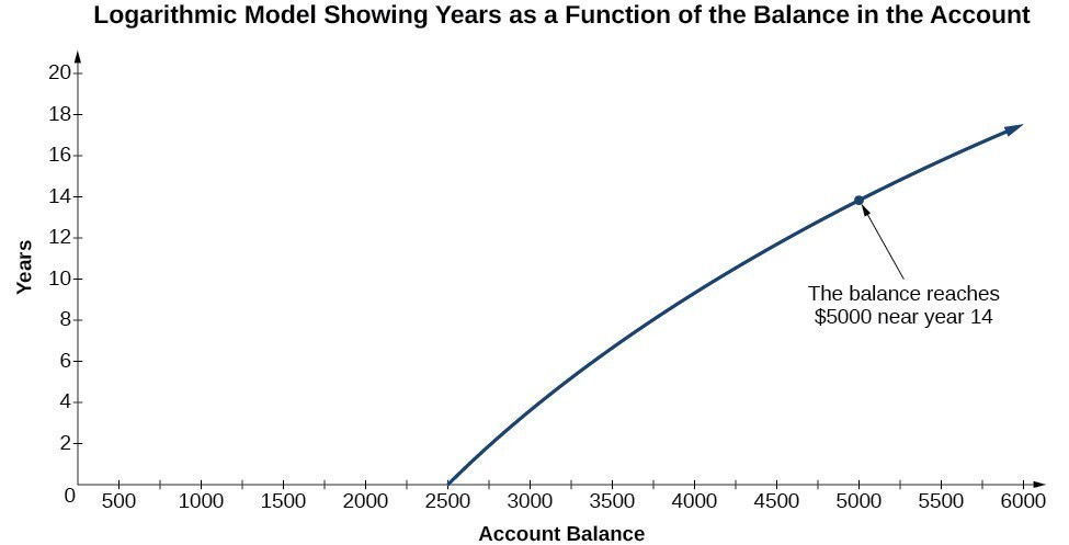
Figure 1
Now that we have a feel for the set of values for which a logarithmic function is defined, we move on to graphing logarithmic functions. The family of logarithmic functions includes the parent function [latex]y={\mathrm{log}}_{b}\left(x\right)[/latex] along with all its transformations: shifts, stretches, compressions, and reflections.
We begin with the parent function [latex]y={\mathrm{log}}_{b}\left(x\right)[/latex]. Because every logarithmic function of this form is the inverse of an exponential function with the form [latex]y={b}^{x}[/latex], their graphs will be reflections of each other across the line [latex]y=x[/latex]. To illustrate this, we can observe the relationship between the input and output values of [latex]y={2}^{x}[/latex] and its equivalent [latex]x={\mathrm{log}}_{2}\left(y\right)[/latex] in the table below.
| x | –3 | –2 | –1 | 0 | 1 | 2 | 3 |
| [latex]{2}^{x}=y[/latex] | [latex]\frac{1}{8}[/latex] | [latex]\frac{1}{4}[/latex] | [latex]\frac{1}{2}[/latex] | 1 | 2 | 4 | 8 |
| [latex]{\mathrm{log}}_{2}\left(y\right)=x[/latex] | –3 | –2 | –1 | 0 | 1 | 2 | 3 |
Using the inputs and outputs from the table above, we can build another table to observe the relationship between points on the graphs of the inverse functions [latex]f\left(x\right)={2}^{x}[/latex] and [latex]g\left(x\right)={\mathrm{log}}_{2}\left(x\right)[/latex].
| [latex]f\left(x\right)={2}^{x}[/latex] | [latex]\left(-3,\frac{1}{8}\right)[/latex] | [latex]\left(-2,\frac{1}{4}\right)[/latex] | [latex]\left(-1,\frac{1}{2}\right)[/latex] | [latex]\left(0,1\right)[/latex] | [latex]\left(1,2\right)[/latex] | [latex]\left(2,4\right)[/latex] | [latex]\left(3,8\right)[/latex] |
| [latex]g\left(x\right)={\mathrm{log}}_{2}\left(x\right)[/latex] | [latex]\left(\frac{1}{8},-3\right)[/latex] | [latex]\left(\frac{1}{4},-2\right)[/latex] | [latex]\left(\frac{1}{2},-1\right)[/latex] | [latex]\left(1,0\right)[/latex] | [latex]\left(2,1\right)[/latex] | [latex]\left(4,2\right)[/latex] | [latex]\left(8,3\right)[/latex] |
As we’d expect, the x– and y-coordinates are reversed for the inverse functions. The figure below shows the graph of f and g.
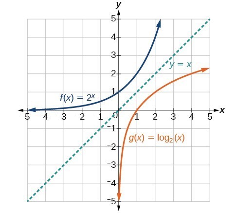
Notice that the graphs of [latex]f\left(x\right)={2}^{x}[/latex] and [latex]g\left(x\right)={\mathrm{log}}_{2}\left(x\right)[/latex] are reflections about the line y = x.
Observe the following from the graph:
- [latex]f\left(x\right)={2}^{x}[/latex] has a y-intercept at [latex]\left(0,1\right)[/latex] and [latex]g\left(x\right)={\mathrm{log}}_{2}\left(x\right)[/latex] has an x-intercept at [latex]\left(1,0\right)[/latex].
- The domain of [latex]f\left(x\right)={2}^{x}[/latex], [latex]\left(-\infty ,\infty \right)[/latex], is the same as the range of [latex]g\left(x\right)={\mathrm{log}}_{2}\left(x\right)[/latex].
- The range of [latex]f\left(x\right)={2}^{x}[/latex], [latex]\left(0,\infty \right)[/latex], is the same as the domain of [latex]g\left(x\right)={\mathrm{log}}_{2}\left(x\right)[/latex].
A General Note: Characteristics of the Graph of the Parent Function, f(x) = logb(x)
For any real number x and constant b > 0, [latex]b\ne 1[/latex], we can see the following characteristics in the graph of [latex]f\left(x\right)={\mathrm{log}}_{b}\left(x\right)[/latex]:
- one-to-one function
- vertical asymptote: x = 0
- domain: [latex]\left(0,\infty \right)[/latex]
- range: [latex]\left(-\infty ,\infty \right)[/latex]
- x-intercept: [latex]\left(1,0\right)[/latex] and key point [latex]\left(b,1\right)[/latex]
- y-intercept: none
- increasing if [latex]b>1[/latex]
- decreasing if 0 < b < 1
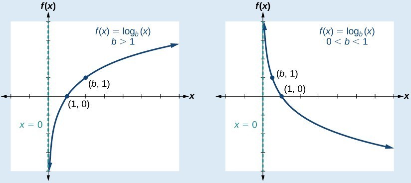
Figure 3
Figure 3 shows how changing the base b in [latex]f\left(x\right)={\mathrm{log}}_{b}\left(x\right)[/latex] can affect the graphs. Observe that the graphs compress vertically as the value of the base increases. (Note: recall that the function [latex]\mathrm{ln}\left(x\right)[/latex] has base [latex]e\approx \text{2}.\text{718.)}[/latex]
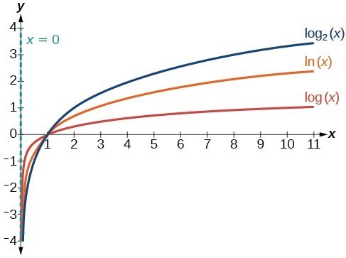
Figure 4. The graphs of three logarithmic functions with different bases, all greater than 1.
In our first example we will graph a logarithmic function of the form [latex]f\left(x\right)={\mathrm{log}}_{b}\left(x\right)[/latex].
Example
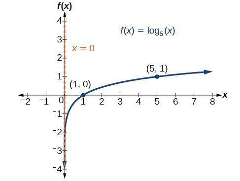
Graph [latex]f\left(x\right)={\mathrm{log}}_{5}\left(x\right)[/latex]. State the domain, range.
How To: Given a logarithmic function with the form [latex]f\left(x\right)={\mathrm{log}}_{b}\left(x\right)[/latex], graph the function.
- Plot the x-intercept, [latex]\left(1,0\right)[/latex].
- Plot the key point [latex]\left(b,1\right)[/latex].
- Draw a smooth curve through the points.
- State the domain, [latex]\left(0,\infty \right)[/latex], the range, [latex]\left(-\infty ,\infty \right)[/latex].
Summary
The inverse of a function can be defined for one-to-one functions. If a function is not one-to-one, it can be possible to restrict it’s domain to make it so. The domain of a function will become the range of it’s inverse. The range of a function will become the domain of it’s inverse. Inverses can be verified using tabular data as well as algebraically.
The base b logarithm of a number is the exponent by which we must raise b to get that number. Logarithmic functions are the inverse of Exponential functions, and it is often easier to understand them through this lens. We can never take the logarithm of a negative number, therefore [latex]{\mathrm{log}}_{b}\left(x\right)=y[/latex] is defined for [latex]b>0[/latex].
Knowing the squares, cubes, and roots of numbers allows us to evaluate many logarithms mentally because the logarithm is an exponent. Logarithms most commonly sue base 10, and often use base e. Logarithms can also be evaluated with most kinds of calculator.
To define the domain of a logarithmic function algebraically, set the argument greater than zero and solve. To plot a logarithmic function, it is easiest to find and plot the x-intercept, and the key point[latex]\left(b,1\right)[/latex].
Earthquake!

A 2×6 plank driven through a ten-ply tire by the tsunami in Whittier, AK.
Joan’s grandpa comes over for dinner every Sunday. Grandpa loves to talk, but it’s really hard to understand him. Also, as he gets older his hearing has been getting worse. Usually Joan tries to find an excuse to be out after dinner on Sundays, but since she had food poisoning on Saturday night, this week she wasn’t feeling like leaving the house.
Grandpa was feeling extra chatty this week and since Joan was a captive audience, she got the full force of his attention. His stories started with the neighbor’s dog who won’t stop barking, then on to his arthritis.
“Joanie, do you know that I think I have arthritis in my ankles because of an earthquake injury?” says Grandpa.
Grandpa went on to tell Joan the story of when he lived in Anchorage, Alaska in the 60’s and lived through the Good Friday earthquake.
The 1964 Alaskan earthquake, also known as the Great Alaskan earthquake, occurred at 5:36 p.m. AST on Good Friday, March 27. Across south-central Alaska, ground fissures, collapsing structures, and earthquake-created tsunamis caused about 139 deaths, some of them being friends of Joan’s grandpa.
Lasting four minutes and thirty-eight seconds, the magnitude 8.5 (Richter scale) [5]megathrust earthquake was the most powerful recorded in North American history, and the second most powerful recorded in world history. Soil liquefaction, fissures, landslides, and other ground failures caused major structural damage in several communities and much damage to property. Post-quake tsunamis severely affected numerous Alaskan communities, as well as people and property in British Columbia, Washington, Oregon, and California. Tsunamis also caused damage in Hawai’i and Japan. Evidence of motion directly related to the earthquake was reported from all over the world.
Surviving the quake inspired Joan’s grandpa to study Geology in college. Joan had heard of the Richter scale before, but didn’t really understand what it meant, so she asked her grandpa.

Charles Richter
He explained that the Richter scale magnitude is expressed in whole numbers and decimal fractions. For example, a magnitude 5.3 might be computed for a moderate earthquake, and a strong earthquake might be rated as magnitude 6.3. Because of the logarithmic basis of the scale, he said, each whole number increase in magnitude represents a tenfold increase in measured amplitude. For example, Grandpa explained, a magnitude 6.3 earthquake corresponds to the release of about 31 times more energy than a magnitude 5.3.[6]
Joan really enjoyed the conversation she had with her grandpa. She had never asked him about his work as a geologist, and she could tell it made him really happy that she did. At least something good emerged out of Joan’s disastrous date and food poisoning fiasco from the night before.
“1964 Quake: The Great Alaska Earthquake” is an eleven minute video created as part of USGS activities acknowledging the fifty year anniversary of the quake on March 27, 2014. The video features USGS geologist George Plafker, who, in the 1960s, correctly interpreted the quake as a subduction zone event. This was a great leap forward in resolving key mechanisms of the developing theory of plate tectonics. The extreme loss of life and destruction from this earthquake and accompanying tsunamis inspired the NOAA Tsunami Warning Centers and the USGS Earthquake Hazards Program.
Candela Citations
- Ex 1: Determine if Two Functions Are Inverses. Authored by: James Sousa (Mathispower4u.com) for Lumen Learning. Located at: https://youtu.be/vObCvTOatfQ. License: CC BY: Attribution
- Ex 2: Determine if Two Functions Are Inverses. Authored by: James Sousa (Mathispower4u.com) for Lumen Learning. Located at: https://youtu.be/hzehBtNmw08. License: CC BY: Attribution
- Ex: Write Exponential Equations as Logarithmic Equations. Authored by: James Sousa (Mathispower4u.com) for Lumen Learning. Located at: https://youtu.be/9_GPPUWEJQQ. License: CC BY: Attribution
- Revision and Adaptation. Provided by: Lumen Learning. License: CC BY: Attribution
- Ex 1: Evaluate Logarithms Without a Calculator - Whole Numbers. Authored by: James Sousa (Mathispower4u.com) for Lumen Learning. Located at: https://youtu.be/dxj5J9OpWGA. License: CC BY: Attribution
- Precalculus. Authored by: Jay Abramson, et al.. Provided by: OpenStax. Located at: http://cnx.org/contents/fd53eae1-fa23-47c7-bb1b-972349835c3c@5.175. License: CC BY: Attribution. License Terms: Download For Free at : http://cnx.org/contents/fd53eae1-fa23-47c7-bb1b-972349835c3c@5.175.
- Ex 1: Composition of Function. Authored by: James Sousa (Mathispower4u.com) . Located at: https://youtu.be/r_LssVS4NHk. License: CC BY: Attribution
- Ex: Function and Inverse Function Values. Authored by: James Sousa (Mathispower4u.com) . Located at: https://youtu.be/IR_1L1mnpvw. License: CC BY: Attribution
- Ex: Write Logarithmic Equations as Exponential Equations. Authored by: James Sousa (Mathispower4u.com) . Located at: https://youtu.be/q9_s0wqhIXU. License: CC BY: Attribution
- Ex: Evaluate Natural Logarithms on the Calculator. Authored by: James Sousa (Mathispower4u.com) . Located at: https://youtu.be/Rpounu3epSc. License: Public Domain: No Known Copyright
- http://earthquake.usgs.gov/earthquakes/eqinthenews/2010/us2010rja6/#summary. Accessed 3/4/2013. ↵
- http://earthquake.usgs.gov/earthquakes/eqinthenews/2011/usc0001xgp/#summary. Accessed 3/4/2013. ↵
- http://earthquake.usgs.gov/earthquakes/eqinthenews/2010/us2010rja6/. Accessed 3/4/2013. ↵
- http://earthquake.usgs.gov/earthquakes/eqinthenews/2011/usc0001xgp/#details. Accessed 3/4/2013. ↵
- "Facts About the 1964 Alaska Earthquake." LiveScience. Accessed August 18, 2016. http://www.livescience.com/44412-1964-alaska-earthquake-facts.html. ↵
- "Measuring the Size of an Earthquake." Measuring the Size of an Earthquake. Accessed August 05, 2016. http://earthquake.usgs.gov/learn/topics/measure.php. ↵
Notice that if we show the coordinate pairs in a table form, the input and output are clearly reversed.