When both the input (independent variable) and the output (dependent variable) are real numbers, a function can be represented by a coordinate graph. The input is plotted on the horizontal x-axis and the output is plotted on the vertical y-axis.

A helpful first step in graphing a function is to make a table of values. This is particularly useful when you don’t know the general shape the function will have. You probably already know that a linear function will be a straight line, but let’s make a table first to see how it can be helpful.

When making a table, it’s a good idea to include negative values, positive values, and zero to ensure that you do have a linear function.

Make a table of values for [latex]f(x)=3x+2[/latex].

Make a two-column table. Label the columns x and f(x).

Choose several values for x and put them as separate rows in the x column. These are YOUR CHOICE – there is no “right” or “wrong” values to pick, just go for it.

Tip: It’s always good to include 0, positive values, and negative values, if you can.

Evaluate the function for each value of x, and write the result in the f(x) column next to the x value you used.

When [latex]x=0[/latex], [latex]f(0)=3(0)+2=2[/latex],

[latex]f(1)=3(1)+2=5[/latex],

[latex]f(−1)=3(−1)+2=−3+2=−1[/latex], and so on.

(Note that your table of values may be different from someone else’s. You may each choose different numbers for x.)

Now that you have a table of values, you can use them to help you draw both the shape and location of the function. Important: The graph of the function will show all possible values of x and the corresponding values of y. This is why the graph is a line and not just the dots that make up the points in our table.

Graph [latex]f(x)=3x+2[/latex].
Using the table of values we created above you can think of f(x) as y, each row forms an ordered pair that you can plot on a coordinate grid.

Plot the points.

Since the points lie on a line, use a straight edge to draw the line. Try to go through each point without moving the straight edge.

Let’s try another one. Before you look at the answer, try to make the table yourself and draw the graph on a piece of paper.

Example

Graph [latex]f(x)=−x+1[/latex].

Show Solution

Start with a table of values. You can choose different values for x, but once again, it’s helpful to include 0, some positive values, and some negative values.

If you think of f(x) as y, each row forms an ordered pair that you can plot on a coordinate grid.

[latex]f(−2)=−(−2)+1=2+1=3\\f(−1)=−(−1)+1=1+1=2\\f(0)=−(0)+1=0+1=1\\f(1)=−(1)+1=−1+1=0\\f(2)=−(2)+1=−2+1=−1[/latex]

x	f(x)
[latex]−2[/latex]	[latex]3[/latex]
[latex]−1[/latex]	[latex]2[/latex]
[latex]0[/latex]	[latex]1[/latex]
[latex]1[/latex]	[latex]0[/latex]
[latex]2[/latex]	[latex]−1[/latex]

Plot the points.

Answer

Since the points lie on a line, use a straight edge to draw the line. Try to go through each point without moving the straight edge.

In the following video we show another example of how to graph a linear function on a set of coordinate axes.

These graphs are representations of a linear function. Remember that a function is a correspondence between two variables, such as x and y.

Graph Quadratic Functions

Quadratic functions can also be graphed. It’s helpful to have an idea what the shape should be, so you can be sure that you’ve chosen enough points to plot as a guide. Let’s start with the most basic quadratic function, [latex]f(x)=x^{2}[/latex].
Graph [latex]f(x)=x^{2}[/latex].
Start with a table of values. Then think of the table as ordered pairs.

Plot the points [latex](-2,4), (-1,1), (0,0), (1,1), (2,4)[/latex]

Since the points are not on a line, you can’t use a straight edge. Connect the points as best you can, using a smooth curve (not a series of straight lines). You may want to find and plot additional points (such as the ones in blue here). Placing arrows on the tips of the lines implies that they continue in that direction forever.

Notice that the shape is like the letter U. This is called a parabola. One-half of the parabola is a mirror image of the other half. The line that goes down the middle is called the line of reflection, in this case that line is they y-axis. The lowest point on this graph is called the vertex.

In the following video we show an example of plotting a quadratic function using a table of values.

The equations for quadratic functions have the form [latex]f(x)=ax^{2}+bx+c[/latex] where [latex] a\ne 0[/latex]. In the basic graph above, [latex]a=1[/latex], [latex]b=0[/latex], and [latex]c=0[/latex].

Changing a changes the width of the parabola and whether it opens up ([latex]a>0[/latex]) or down ([latex]a<0[/latex]). If a is positive, the vertex is the lowest point, if a is negative, the vertex is the highest point. In the following example, we show how changing the value of a will affect the graph of the function.

Example

Match the following functions with their graph.

a) [latex] \displaystyle f(x)=3{{x}^{2}}[/latex]

b) [latex] \displaystyle f(x)=-3{{x}^{2}}[/latex]

c)[latex] \displaystyle f(x)=\frac{1}{2}{{x}^{2}}[/latex]

a)

b)

c)

Show Answer

Function a) [latex] \displaystyle f(x)=3{{x}^{2}}[/latex] means that inputs are squared and then multiplied by three, so the outputs will be greater than they would have been for [latex]f(x)=x^2[/latex].  This results in a parabola that has been squeezed, so the graph b) is the best match for this function.

Function b) [latex] \displaystyle f(x)=-3{{x}^{2}}[/latex] means that inputs are squared and then multiplied by negative three, so the outputs will be greater than they would have been for [latex]f(x)=x^2[/latex] so graph a)  is the best match for this function.

Function c) [latex] \displaystyle f(x)=\frac{1}{2}{{x}^{2}}[/latex] means that inputs are squared then multiplied by [latex]\frac{1}{2}[/latex], so the outputs are less than they would be for [latex]f(x)=x^2[/latex].  This results in a parabola that has been opened wider than[latex]f(x)=x^2[/latex]. Graph c) is the best match for this function.

Answer

Function a) matches graph b)

Function b) matches graph a)

Function c) matches graph c)

If there is no b term, changing c moves the parabola up or down so that the y intercept is (0, c). In the next example we show how changes to c affect the graph of the function.

Example

Match the following functions with their graph.

a) [latex] \displaystyle f(x)={{x}^{2}}+3[/latex]

b) [latex] \displaystyle f(x)={{x}^{2}}-3[/latex]

a)

b)

Show Answer

Function a) [latex] \displaystyle f(x)={{x}^{2}}+3[/latex] means square the inputs then add three, so every output will be moved up 3 units. the graph that matches this function best is b)

Function b) [latex] \displaystyle f(x)={{x}^{2}}-3[/latex]  means square the inputs then subtract three, so every output will be moved down 3 units. the graph that matches this function best is a)

Changing b moves the line of reflection, which is the vertical line that passes through the vertex ( the high or low point) of the parabola. It may help to know how calculate the vertex of a parabola to understand how changing the value of b in a function will change it’s graph.

To find the vertex of the parabola, use the formula [latex] \displaystyle \left( \frac{-b}{2a},f\left( \frac{-b}{2a} \right) \right)[/latex].

For example, if the function in consideration is [latex]f(x)=2x^2-3x+4[/latex], to find the vertex, first calculate [latex]\frac{-b}{2a}[/latex]

a = 2, and b = -3, therefore [latex]\frac{-b}{2a}=\frac{-(-3)}{2(2)}=\frac{3}{4}[/latex].

This is the x value of the vertex.

Now evaluate the function at [latex]x =\frac{3}{4}[/latex] to get the corresponding y-value for the vertex.

[latex]f\left( \frac{-b}{2a} \right)=2\left(\frac{3}{4}\right)^2-3\left(\frac{3}{4}\right)+4=2\left(\frac{9}{16}\right)-4+4=\frac{9}{8}[/latex].

The vertex is at the point [latex]\left(\frac{3}{4},\frac{9}{8}\right)[/latex].  This means that the vertical line of reflection passes through this point as well.  It is not easy to tell how changing the values for b will change the graph of a quadratic function, but if you find the vertex, you can tell how the graph will change.

In the next example we show how changing b can change the graph of the quadratic function.

Example

Match the following functions with their graph.

a) [latex] \displaystyle f(x)={{x}^{2}}+2x[/latex]

b) [latex] \displaystyle f(x)={{x}^{2}}-2x[/latex]

a)

b)

Show Answer

Find the vertex of function a)[latex] \displaystyle f(x)={{x}^{2}}+2x[/latex].

a = 1, b = 2

x-value:

[latex]\frac{-b}{2a}=\frac{-2}{2(1)}=-1[/latex]

y-value:

[latex]f\left(\frac{-b}{2a}\right)=\left(-1)^2+2\left(-1)=1-2=-1[/latex].

Vertex = [latex]\left(-1,-1)[/latex], which means the graph that best fits this function is a)

Find the vertex of function b)[latex] \displaystyle f(x)={{x}^{2}}-2x[/latex].

a = 1, b = -2

x-value:

[latex]\frac{-b}{2a}=\frac{2}{2(1)}=1[/latex]

y-value:

[latex]f\left(\frac{-b}{2a}\right)=\left(1)^2-2\left(1)=1-2=-1[/latex].

Vertex = [latex]\left(1,-1)[/latex], which means the graph that best fits this function is b)

Note that the vertex can change if the value for c changes because the y-value of the vertex is calculated by substituting the x-value into the function. Here is a summary of how the changes to the values for a, b, and, c of a quadratic function can change it’s graph.

Properties of a Parabola

For [latex] \displaystyle f(x)=a{{x}^{2}}+bx+c[/latex], where a, b, and c are real numbers.

• The parabola opens upward if a > 0 and downward if a < 0.
• a changes the width of the parabola. The parabola gets narrower if |a| is > 1 and wider if |a|<1.
• The vertex depends on the values of a, b, and c. The vertex is [latex]\left(\frac{-b}{2a},f\left( \frac{-b}{2a}\right)\right)[/latex].

In the last example we show how you can use the properties of a parabola to help you make a graph without having to calculate an exhaustive table of values.

Example

Graph [latex]f(x)=−2x^{2}+3x–3[/latex].

Show Solution

Before making a table of values, look at the values of a and c to get a general idea of what the graph should look like.

[latex]a=−2[/latex], so the graph will open down and be thinner than [latex]f(x)=x^{2}[/latex].

[latex]c=−3[/latex], so it will move to intercept the y-axis at [latex](0,−3)[/latex].

To find the vertex of the parabola, use the formula [latex] \displaystyle \left( \frac{-b}{2a},f\left( \frac{-b}{2a} \right) \right)[/latex]. Finding the vertex may make graphing the parabola easier.

[latex]\text{Vertex }\text{formula}=\left( \frac{-b}{2a},f\left( \frac{-b}{2a} \right) \right)[/latex]

x-coordinate of vertex:

[latex] \displaystyle \frac{-b}{2a}=\frac{-(3)}{2(-2)}=\frac{-3}{-4}=\frac{3}{4}[/latex]

y-coordinate of vertex:

[latex] \displaystyle \begin{array}{l}f\left( \frac{-b}{2a} \right)=f\left( \frac{3}{4} \right)\\\,\,\,f\left( \frac{3}{4} \right)=-2{{\left( \frac{3}{4} \right)}^{2}}+3\left( \frac{3}{4} \right)-3\\\,\,\,\,\,\,\,\,\,\,\,\,\,\,\,\,\,\,=-2\left( \frac{9}{16} \right)+\frac{9}{4}-3\\\,\,\,\,\,\,\,\,\,\,\,\,\,\,\,\,\,\,=\frac{-18}{16}+\frac{9}{4}-3\\\,\,\,\,\,\,\,\,\,\,\,\,\,\,\,\,\,\,=\frac{-9}{8}+\frac{18}{8}-\frac{24}{8}\\\,\,\,\,\,\,\,\,\,\,\,\,\,\,\,\,\,\,=-\frac{15}{8}\end{array}\\[/latex]

Vertex: [latex] \displaystyle \left( \frac{3}{4},-\frac{15}{8} \right)\\[/latex]

Use the vertex, [latex] \displaystyle \left( \frac{3}{4},-\frac{15}{8} \right)\\[/latex], and the properties you described to get a general idea of the shape of the graph. You can create a table of values to verify your graph. Notice that in this table, the x values increase. The y values increase and then start to decrease again. That indicates a parabola.

x	f(x)
[latex]−2[/latex]	[latex]−17[/latex]
[latex]−1[/latex]	[latex]−8[/latex]
[latex]0[/latex]	[latex]−3[/latex]
[latex]1[/latex]	[latex]−2[/latex]
[latex]2[/latex]	[latex]−5[/latex]

Answer

Connect the points as best you can, using a smooth curve. Remember that the parabola is two mirror images, so if your points don’t have pairs with the same value, you may want to include additional points (such as the ones in blue here). Plot points on either side of the vertex.

[latex]x=\frac{1}{2}[/latex] and [latex]x=\frac{3}{2}[/latex] are good values to include.

The following video shows another example of plotting a quadratic function using the vertex.

Creating a graph of a function is one way to understand the relationship between the inputs and outputs of that function. Creating a graph can be done by choosing values for x, finding the corresponding y values, and plotting them. However, it helps to understand the basic shape of the function. Knowing the effect of changes to the basic function equation is also helpful.

One common shape you will see is a parabola. Parabolas have the equation [latex]f(x)=ax^{2}+bx+c[/latex], where a, b, and c are real numbers and [latex]a\ne0[/latex]. The value of a determines the width and the direction of the parabola, while the vertex depends on the values of a, b, and c. The vertex is [latex] \displaystyle \left( \frac{-b}{2a},f\left( \frac{-b}{2a} \right) \right)\\[/latex].

Graph Radical Functions

You can also graph radical functions (such as square root functions) by choosing values for x and finding points that will be on the graph. Again, it’s helpful to have some idea about what the graph will look like.

Think about the basic square root function, [latex]f(x)=\sqrt{x}[/latex]. Let’s take a look at a table of values for x and y and then graph the function. (Notice that all the values for x in the table are perfect squares. Since you are taking the square root of x, using perfect squares makes more sense than just finding the square roots of 0, 1, 2, 3, 4, etc.)

Recall that x can never be negative because when you square a real number, the result is always positive. For example, [latex]\sqrt{49}[/latex], this means “find the number whose square is 49.”  Since there is no real number that we can square and get a negative, the function [latex]f(x)=\sqrt{x}[/latex] will be defined for [latex]x>0[/latex].

Take a look at the graph.

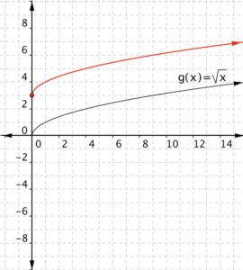
As with parabolas, multiplying and adding numbers makes some changes, but the basic shape is still the same. Here are some examples. 

Multiplying [latex]\sqrt{x}[/latex] by a positive value changes the width of the half-parabola. Multiplying [latex]\sqrt{x}[/latex] by a negative number gives you the other half of a horizontal parabola.

In the following example we will show how multiplying a radical function by a constant can change the shape of the graph.

Example

Match each of the following functions to the graph that it represents.

a) [latex]f(x)=-\sqrt{x}[/latex]

b)[latex]f(x)=2\sqrt{x}[/latex]

c) [latex]f(x)=\frac{1}{2}\sqrt{x}[/latex]

a)

b)

c)

Show Answer

Function a) [latex]f(x)=-\sqrt{x}[/latex] means that all the outputs will be negative – the function is the negative of the square roots of the input.  This will give the other half of the parabola on it’s side.  Therefore the graph

goes with the function [latex]f(x)=-\sqrt{x}[/latex]

Function b)[latex]f(x)=2\sqrt{x}[/latex] means take the square root of all the inputs, then multiply by two, so the outputs will be larger than the outputs for [latex]\sqrt{x}[/latex].  The graph

goes with the function [latex]f(x)=2\sqrt{x}[/latex]

Function c) [latex]f(x)=\frac{1}{2}\sqrt{x}[/latex] means take the squat=re root of the inputs then multiply by [latex]\frac{1}{2}[/latex]. The outputs will be smaller than the outputs for [latex]\sqrt{x}[/latex]. The graph

goes with the function [latex]f(x)=\frac{1}{2}\sqrt{x}[/latex].

Answer

Function a) goes with graph b)

Function b) goes with graph a)

Function c) goes with graph c)

Adding a value outside the radical moves the graph up or down. Think about it as adding the value to the basic y value of [latex] \sqrt{x}[/latex], so a positive value added moves the graph up.

Example

Match each of the following functions to the graph that it represents.

a) [latex] f(x)=\sqrt{x}+3[/latex]

b)[latex] f(x)=\sqrt{x}-2[/latex]

a)

b)

Show Answer

Function a) [latex] f(x)=\sqrt{x}+3[/latex] means take the square root of all the inputs and add three, so the out puts will be greater than those for [latex]\sqrt{x}[/latex], therefore the graph that goes with this function is

Function b) [latex]f(x)=\sqrt{x}-2[/latex] means take the square root of the input then subtract two. The outputs will be less than those for [latex]\sqrt{x}[/latex], therefore the graph that goes with this function is

Answer

Function a) goes with graph b)

Function b) goes with graph a)

Adding a value inside the radical moves the graph left or right. Think about it as adding a value to x before you take the square root—so the y value gets moved to a different x value. For example, for [latex]f(x)=\sqrt{x}[/latex], the square root is 3 if [latex]x=9[/latex]. For[latex]f(x)=\sqrt{x+1}[/latex], the square root is 3 when [latex]x+1[/latex] is 9, so x is 8. Changing x to [latex]x+1[/latex] shifts the graph to the left by 1 unit (from 9 to 8). Changing x to [latex]x−2[/latex] shifts the graph to the right by 2 units.

Example

Match each of the following functions to the graph that it represents.

a) [latex]f(x)=\sqrt{x+1}[/latex]

b)[latex]f(x)=\sqrt{x-2}[/latex]

a)

b)

Show Answer

Function a) [latex]f(x)=\sqrt{x+1}[/latex] adds one to the inputs before the square root is taken.  The outputs will be greater, so it ends up looking like a shift to the left. The graph that matches this function is

Function b) [latex]f(x)=\sqrt{x-2}[/latex] means subtract before the square root is taken.  This makes the outputs less than they would be for the standard [latex]\sqrt{x}[/latex], and looks like a shift to the right. the graph that matches this function is

Answer

Function a) matches graph b)

Function b) matches graph a)

Notice that as x gets greater, adding or subtracting a number inside the square root has less of an effect on the value of y!

In the next example we will combine some of the changes that we have seen into one function.

Example

Graph [latex] f(x)=-2+\sqrt{x-1}[/latex].

Show Solution

Before making a table of values, look at the function equation to get a general idea what the graph should look like.

Inside the square root, you’re subtracting 1, so the graph will move to the right 1 from the basic [latex] f(x)=\sqrt{x}[/latex] graph.

You’re also adding [latex]−2[/latex] outside the square root, so the graph will move down two from the basic [latex] f(x)=\sqrt{x}[/latex] graph.

Create a table of values. Choose values that will make your calculations easy. You want [latex]x–1[/latex] to be a perfect square (0, 1, 4, 9, and so on) so you can take the square root.

x	f(x)
[latex]1[/latex]	[latex]−2[/latex]
[latex]2[/latex]	[latex]−1[/latex]
[latex]5[/latex]	[latex]0[/latex]
[latex]10[/latex]	[latex]1[/latex]

Since values of x less than 1 makes the value inside the square root negative, there will be no points on the coordinate graph to the left of [latex]x=1[/latex]. There is no need to choose x values less than 1 for your table!

Use the table pairs to plot points.

Connect the points as best you can, using a smooth curve.

Answer

Identify a One-to-One Function

Remember that in a function, the input value must have one and only one value for the output. There is a name for the set of input values and another name for the set of output values for a function. The set of input values is called the domain of the function. And the set of output values is called the range of the function.

In the first example we remind you how to define domain and range using a table of values.

In the following video we show another example of finding domain and range from tabular data.

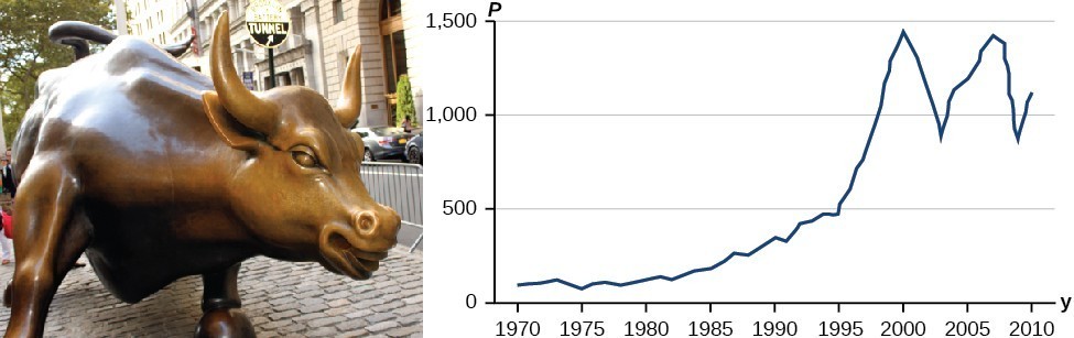
Some functions have a given output value that corresponds to two or more input values. For example, in the following stock chart the stock price was $1000 on five different dates, meaning that there were five different input values that all resulted in the same output value of $1000.

However, some functions have only one input value for each output value, as well as having only one output for each input. We call these functions one-to-one functions. As an example, consider a school that uses only letter grades and decimal equivalents, as listed in.

This grading system represents a one-to-one function, because each letter input yields one particular grade point average output and each grade point average corresponds to one input letter.

To visualize this concept, let’s look again at the two simple functions sketched in (a)and (b) of Figure 10.

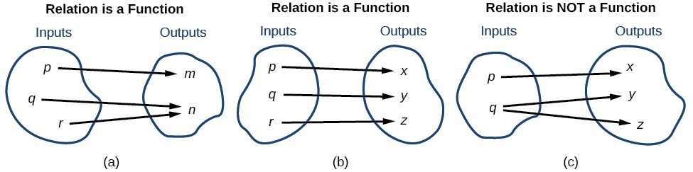
Figure 10

The function in part (a) shows a relationship that is not a one-to-one function because inputs [latex]q[/latex] and [latex]r[/latex] both give output [latex]n[/latex]. The function in part (b) shows a relationship that is a one-to-one function because each input is associated with a single output.

In the following video, we show an example of using tables of values to determine whether a function is one-to-one.

Using the Horizontal Line Test

An easy way to determine whether a function is a one-to-one function is to use the horizontal line test on the graph of the function.  To do this, draw horizontal lines through the graph. If any horizontal line intersects the graph more than once, then the graph does not represent a one-to-one function.

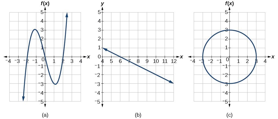
Exercises

For the following graphs, determine which represent one-to-one functions.

Show Answer

The function in (a) is not one-to-one. Using the horizontal line test, as shown below, it intersects the graph of the function at two points (and we can even find horizontal lines that intersect it at three points.)

 

The function in (b) is one-to-one. Any horizontal line will intersect a diagonal line at most once.

The function (c) is not one-to-one, and is in fact not a function.

The following video provides another example of using the horizontal line test to determine whether a graph represents a one-to-one function.

Summary

In real life and in algebra, different variables are often linked. When a change in value of one variable causes a change in the value of another variable, their interaction is called a relation. A relation has an input value which corresponds to an output value. When each input value has one and only one output value, that relation is a function. Functions can be written as ordered pairs, tables, or graphs. The set of input values is called the domain, and the set of output values is called the range.