Learning Objectives
- Apply table styles.
One very common task in Excel is to format a table with a particular style. The controls for table styles are found in the Styles group of the ribbon under the Home tab.
There are many default table styles within Excel, as shown in the screenshot below. Among other uses, styles let you apply color schemes to tables that can make them more readable. In order to apply a particular table style:
- Select all the cells that belong in your table.
- Click on the “Format as Table” button.
- Choose which table style to apply.
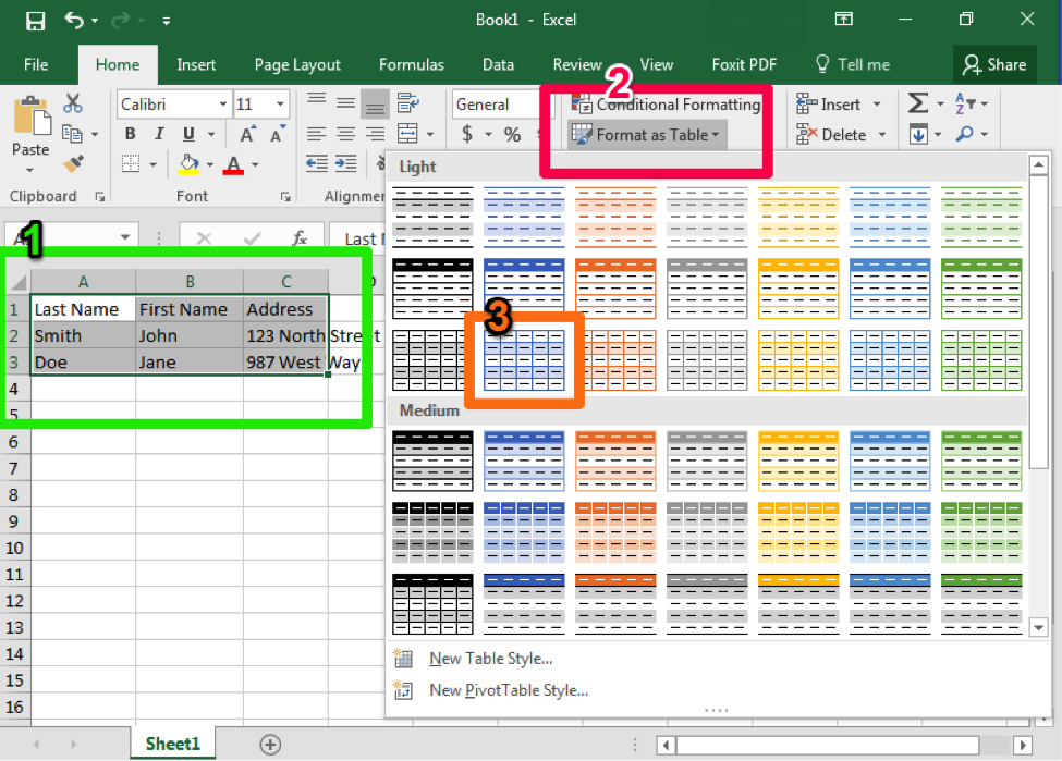
Select all the cells that belong in your table. Click on the “Format as Table” button. Choose which table style to apply.
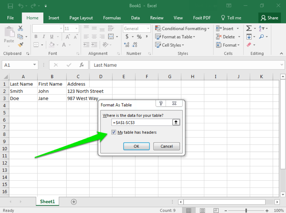
In the screenshot example, each column is a particular type of information (Last name, First Name, Address). These are known as headers. When applying the table style, be sure to check the box if your table has headers that you have already entered.
Practice Question
Practice Question
Your final table would look something like the table below using the options shown in the screenshots.

Candela Citations
- Styles within Excel. Authored by: Shelli Carter. Provided by: Lumen Learning. License: CC BY: Attribution