Discuss the ways populations evolve

All life on Earth is related. Evolutionary theory states that humans, beetles, plants, and bacteria all share a common ancestor, but that millions of years of evolution have shaped each of these organisms into the forms seen today. Scientists consider evolution a key concept to understanding life. Natural selection is one of the most dominant evolutionary forces. Natural selection acts to promote traits and behaviors that increase an organism’s chances of survival and reproduction, while eliminating those traits and behaviors that are to the organism’s detriment. But natural selection can only, as its name implies, select—it cannot create. The introduction of novel traits and behaviors falls on the shoulders of another evolutionary force—mutation. Mutation and other sources of variation among individuals, as well as the evolutionary forces that act upon them, alter populations and species. This combination of processes has led to the world of life we see today.

Population Genetics

Recall that a gene for a particular character may have several alleles, or variants, that code for different traits associated with that character. For example, in the ABO blood type system in humans, three alleles determine the particular blood-type protein on the surface of red blood cells. Each individual in a population of diploid organisms can only carry two alleles for a particular gene, but more than two may be present in the individuals that make up the population. Mendel followed alleles as they were inherited from parent to offspring. In the early twentieth century, biologists in a field of study known as population genetics began to study how selective forces change a population through changes in allele and genotypic frequencies.

The allele frequency (or gene frequency) is the rate at which a specific allele appears within a population. Until now we have discussed evolution as a change in the characteristics of a population of organisms, but behind that phenotypic change is genetic change. In population genetics, the term evolution is defined as a change in the frequency of an allele in a population. Using the ABO blood type system as an example, the frequency of one of the alleles, I^A, is the number of copies of that allele divided by all the copies of the ABO gene in the population. For example, a study in Jordan^[1] found a frequency of I^A to be 26.1 percent. The I^Band I⁰ alleles made up 13.4 percent and 60.5 percent of the alleles respectively, and all of the frequencies added up to 100 percent. A change in this frequency over time would constitute evolution in the population.

The allele frequency within a given population can change depending on environmental factors; therefore, certain alleles become more widespread than others during the process of natural selection. Natural selection can alter the population’s genetic makeup; for example, if a given allele confers a phenotype that allows an individual to better survive or have more offspring. Because many of those offspring will also carry the beneficial allele, and often the corresponding phenotype, they will have more offspring of their own that also carry the allele, thus, perpetuating the cycle. Over time, the allele will spread throughout the population. Some alleles will quickly become fixed in this way, meaning that every individual of the population will carry the allele, while detrimental mutations may be swiftly eliminated if derived from a dominant allele from the gene pool. The gene pool is the sum of all the alleles in a population.

Sometimes, allele frequencies within a population change randomly with no advantage to the population over existing allele frequencies. This phenomenon is called genetic drift. Natural selection and genetic drift usually occur simultaneously in populations and are not isolated events. It is hard to determine which process dominates because it is often nearly impossible to determine the cause of change in allele frequencies at each occurrence. An event that initiates an allele frequency change in an isolated part of the population, which is not typical of the original population, is called the founder effect. Natural selection, random drift, and founder effects can lead to significant changes in the genome of a population.

Hardy-Weinberg Principle of Equilibrium

In the early twentieth century, English mathematician Godfrey Hardy and German physician Wilhelm Weinberg stated the principle of equilibrium to describe the genetic makeup of a population. The theory, which later became known as the Hardy-Weinberg principle of equilibrium, states that a population’s allele and genotype frequencies are inherently stable— unless some kind of evolutionary force is acting upon the population, neither the allele nor the genotypic frequencies would change. The Hardy-Weinberg principle assumes conditions with no mutations, migration, emigration, or selective pressure for or against genotype, plus an infinite population; while no population can satisfy those conditions, the principle offers a useful model against which to compare real population changes.

Working under this theory, population geneticists represent different alleles as different variables in their mathematical models. The variable p, for example, often represents the frequency of a particular allele, say Y for the trait of yellow in Mendel’s peas, while the variable q represents the frequency of y alleles that confer the color green. If these are the only two possible alleles for a given locus in the population, p + q = 1. In other words, all the p alleles and all the q alleles make up all of the alleles for that locus that are found in the population.

But what ultimately interests most biologists is not the frequencies of different alleles, but the frequencies of the resulting genotypes, known as the population’s genetic structure, from which scientists can surmise the distribution of phenotypes. If the phenotype is observed, only the genotype of the homozygous recessive alleles can be known; the calculations provide an estimate of the remaining genotypes. Since each individual carries two alleles per gene, if the allele frequencies (p and q) are known, predicting the frequencies of these genotypes is a simple mathematical calculation to determine the probability of getting these genotypes if two alleles are drawn at random from the gene pool. So in the above scenario, an individual pea plant could be pp (YY), and thus produce yellow peas; pq (Yy), also yellow; or qq (yy), and thus producing green peas (Figure 1). In other words, the frequency of pp individuals is simply p²; the frequency of pq individuals is 2pq; and the frequency of qq individuals is q². And, again, if p and q are the only two possible alleles for a given trait in the population, these genotypes frequencies will sum to one: p²+ 2pq + q² = 1.

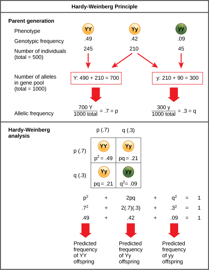
Figure 1. When populations are in the Hardy-Weinberg equilibrium, the allelic frequency is stable from generation to generation and the distribution of alleles can be determined from the Hardy-Weinberg equation. If the allelic frequency measured in the field differs from the predicted value, scientists can make inferences about what evolutionary forces are at play.

In theory, if a population is at equilibrium—that is, there are no evolutionary forces acting upon it—generation after generation would have the same gene pool and genetic structure, and these equations would all hold true all of the time. Of course, even Hardy and Weinberg recognized that no natural population is immune to evolution. Populations in nature are constantly changing in genetic makeup due to drift, mutation, possibly migration, and selection. As a result, the only way to determine the exact distribution of phenotypes in a population is to go out and count them. But the Hardy-Weinberg principle gives scientists a mathematical baseline of a non-evolving population to which they can compare evolving populations and thereby infer what evolutionary forces might be at play. If the frequencies of alleles or genotypes deviate from the value expected from the Hardy-Weinberg equation, then the population is evolving.

Genetic Variation and Drift

Figure 2. The distribution of phenotypes in this litter of kittens illustrates population variation. (credit: Pieter Lanser)

Individuals of a population often display different phenotypes, or express different alleles of a particular gene, referred to as polymorphisms. Populations with two or more variations of particular characteristics are called polymorphic. The distribution of phenotypes among individuals, known as the population variation, is influenced by a number of factors, including the population’s genetic structure and the environment (Figure 2). Understanding the sources of a phenotypic variation in a population is important for determining how a population will evolve in response to different evolutionary pressures.

Genetic Variance

Natural selection and some of the other evolutionary forces can only act on heritable traits, namely an organism’s genetic code. Because alleles are passed from parent to offspring, those that confer beneficial traits or behaviors may be selected for, while deleterious alleles may be selected against. Acquired traits, for the most part, are not heritable. For example, if an athlete works out in the gym every day, building up muscle strength, the athlete’s offspring will not necessarily grow up to be a body builder. If there is a genetic basis for the ability to run fast, on the other hand, this may be passed to a child.

Heritability is the fraction of phenotype variation that can be attributed to genetic differences, or genetic variance, among individuals in a population. The greater the hereditability of a population’s phenotypic variation, the more susceptible it is to the evolutionary forces that act on heritable variation.

The diversity of alleles and genotypes within a population is called genetic variance. When scientists are involved in the breeding of a species, such as with animals in zoos and nature preserves, they try to increase a population’s genetic variance to preserve as much of the phenotypic diversity as they can. This also helps reduce the risks associated with inbreeding, the mating of closely related individuals, which can have the undesirable effect of bringing together deleterious recessive mutations that can cause abnormalities and susceptibility to disease. For example, a disease that is caused by a rare, recessive allele might exist in a population, but it will only manifest itself when an individual carries two copies of the allele. Because the allele is rare in a normal, healthy population with unrestricted habitat, the chance that two carriers will mate is low, and even then, only 25 percent of their offspring will inherit the disease allele from both parents. While it is likely to happen at some point, it will not happen frequently enough for natural selection to be able to swiftly eliminate the allele from the population, and as a result, the allele will be maintained at low levels in the gene pool. However, if a family of carriers begins to interbreed with each other, this will dramatically increase the likelihood of two carriers mating and eventually producing diseased offspring, a phenomenon known as inbreeding depression.

Changes in allele frequencies that are identified in a population can shed light on how it is evolving. In addition to natural selection, there are other evolutionary forces that could be in play: genetic drift, gene flow, mutation, nonrandom mating, and environmental variances.

Genetic Drift

The theory of natural selection stems from the observation that some individuals in a population are more likely to survive longer and have more offspring than others; thus, they will pass on more of their genes to the next generation. A big, powerful male gorilla, for example, is much more likely than a smaller, weaker one to become the population’s silverback, the pack’s leader who mates far more than the other males of the group. The pack leader will father more offspring, who share half of his genes, and are likely to also grow bigger and stronger like their father. Over time, the genes for bigger size will increase in frequency in the population, and the population will, as a result, grow larger on average. That is, this would occur if this particular selection pressure, or driving selective force, were the only one acting on the population. In other examples, better camouflage or a stronger resistance to drought might pose a selection pressure.

Another way a population’s allele and genotype frequencies can change is genetic drift (Figure 3), which is simply the effect of chance. By chance, some individuals will have more offspring than others—not due to an advantage conferred by some genetically-encoded trait, but just because one male happened to be in the right place at the right time (when the receptive female walked by) or because the other one happened to be in the wrong place at the wrong time (when a fox was hunting).

Figure 3. Click for a larger image. Genetic drift in a population can lead to the elimination of an allele from a population by chance. In this example, rabbits with the brown coat color allele (B) are dominant over rabbits with the white coat color allele (b). In the first generation, the two alleles occur with equal frequency in the population, resulting in p and q values of .5. Only half of the individuals reproduce, resulting in a second generation with p and q values of .7 and .3, respectively. Only two individuals in the second generation reproduce, and by chance these individuals are homozygous dominant for brown coat color. As a result, in the third generation the recessive b allele is lost.

Small populations are more susceptible to the forces of genetic drift. Large populations, on the other hand, are buffered against the effects of chance. If one individual of a population of 10 individuals happens to die at a young age before it leaves any offspring to the next generation, all of its genes—1/10 of the population’s gene pool—will be suddenly lost. In a population of 100, that’s only 1 percent of the overall gene pool; therefore, it is much less impactful on the population’s genetic structure.

Watch this animation of random sampling and genetic drift in action:

Bottleneck Effect

Figure 4. A chance event or catastrophe can reduce the genetic variability within a population.

Genetic drift can also be magnified by natural events, such as a natural disaster that kills—at random—a large portion of the population. Known as the bottleneck effect, it results in a large portion of the genome suddenly being wiped out (Figure 4). In one fell swoop, the genetic structure of the survivors becomes the genetic structure of the entire population, which may be very different from the pre-disaster population.

Founder Effect

Another scenario in which populations might experience a strong influence of genetic drift is if some portion of the population leaves to start a new population in a new location or if a population gets divided by a physical barrier of some kind. In this situation, those individuals are unlikely to be representative of the entire population, which results in the founder effect. The founder effect occurs when the genetic structure changes to match that of the new population’s founding fathers and mothers. The founder effect is believed to have been a key factor in the genetic history of the Afrikaner population of Dutch settlers in South Africa, as evidenced by mutations that are common in Afrikaners but rare in most other populations. This is likely due to the fact that a higher-than-normal proportion of the founding colonists carried these mutations. As a result, the population expresses unusually high incidences of Huntington’s disease (HD) and Fanconi anemia (FA), a genetic disorder known to cause blood marrow and congenital abnormalities—even cancer.

Gene Flow

Figure 5. Gene flow can occur when an individual travels from one geographic location to another.

Another important evolutionary force is gene flow: the flow of alleles in and out of a population due to the migration of individuals or gametes (Figure 5). While some populations are fairly stable, others experience more flux. Many plants, for example, send their pollen far and wide, by wind or by bird, to pollinate other populations of the same species some distance away. Even a population that may initially appear to be stable, such as a pride of lions, can experience its fair share of immigration and emigration as developing males leave their mothers to seek out a new pride with genetically unrelated females. This variable flow of individuals in and out of the group not only changes the gene structure of the population, but it can also introduce new genetic variation to populations in different geological locations and habitats.

Mutation

Mutations are changes to an organism’s DNA and are an important driver of diversity in populations. Species evolve because of the accumulation of mutations that occur over time. The appearance of new mutations is the most common way to introduce novel genotypic and phenotypic variance. Some mutations are unfavorable or harmful and are quickly eliminated from the population by natural selection. Others are beneficial and will spread through the population. Whether or not a mutation is beneficial or harmful is determined by whether it helps an organism survive to sexual maturity and reproduce. Some mutations do not do anything and can linger, unaffected by natural selection, in the genome. Some can have a dramatic effect on a gene and the resulting phenotype.

Nonrandom Mating

If individuals nonrandomly mate with their peers, the result can be a changing population. There are many reasons nonrandom mating occurs. One reason is simple mate choice; for example, female peahens may prefer peacocks with bigger, brighter tails. Traits that lead to more matings for an individual become selected for by natural selection. One common form of mate choice, called assortative mating, is an individual’s preference to mate with partners who are phenotypically similar to themselves.

Another cause of nonrandom mating is physical location. This is especially true in large populations spread over large geographic distances where not all individuals will have equal access to one another. Some might be miles apart through woods or over rough terrain, while others might live immediately nearby.

Environmental Variance

Figure 6. The sex of the American alligator (Alligator mississippiensis) is determined by the temperature at which the eggs are incubated. Eggs incubated at 30°C produce females, and eggs incubated at 33°C produce males. (credit: Steve Hillebrand, USFWS)

Genes are not the only players involved in determining population variation. Phenotypes are also influenced by other factors, such as the environment (Figure 6). A beachgoer is likely to have darker skin than a city dweller, for example, due to regular exposure to the sun, an environmental factor. Some major characteristics, such as sex, are determined by the environment for some species. For example, some turtles and other reptiles have temperature-dependent sex determination (TSD). TSD means that individuals develop into males if their eggs are incubated within a certain temperature range, or females at a different temperature range.

Geographic separation between populations can lead to differences in the phenotypic variation between those populations. Such geographical variation is seen between most populations and can be significant. One type of geographic variation, called a cline, can be seen as populations of a given species vary gradually across an ecological gradient. Species of warm-blooded animals, for example, tend to have larger bodies in the cooler climates closer to the earth’s poles, allowing them to better conserve heat. This is considered a latitudinal cline. Alternatively, flowering plants tend to bloom at different times depending on where they are along the slope of a mountain, known as an altitudinal cline.

If there is gene flow between the populations, the individuals will likely show gradual differences in phenotype along the cline. Restricted gene flow, on the other hand, can lead to abrupt differences, even speciation.

Adaptive Evolution

Natural selection only acts on the population’s heritable traits: selecting for beneficial alleles and thus increasing their frequency in the population, while selecting against deleterious alleles and thereby decreasing their frequency—a process known as adaptive evolution. Natural selection does not act on individual alleles, however, but on entire organisms. An individual may carry a very beneficial genotype with a resulting phenotype that, for example, increases the ability to reproduce (fecundity), but if that same individual also carries an allele that results in a fatal childhood disease, that fecundity phenotype will not be passed on to the next generation because the individual will not live to reach reproductive age. Natural selection acts at the level of the individual; it selects for individuals with greater contributions to the gene pool of the next generation, known as an organism’s evolutionary (Darwinian) fitness.

Fitness is often quantifiable and is measured by scientists in the field. However, it is not the absolute fitness of an individual that counts, but rather how it compares to the other organisms in the population. This concept, called relative fitness, allows researchers to determine which individuals are contributing additional offspring to the next generation, and thus, how the population might evolve.

There are several ways selection can affect population variation: stabilizing selection, directional selection, diversifying selection, frequency-dependent selection, and sexual selection. As natural selection influences the allele frequencies in a population, individuals can either become more or less genetically similar and the phenotypes displayed can become more similar or more disparate.

Stabilizing Selection

If natural selection favors an average phenotype, selecting against extreme variation, the population will undergo stabilizing selection (Figure 7). In a population of mice that live in the woods, for example, natural selection is likely to favor individuals that best blend in with the forest floor and are less likely to be spotted by predators. Assuming the ground is a fairly consistent shade of brown, those mice whose fur is most closely matched to that color will be most likely to survive and reproduce, passing on their genes for their brown coat. Mice that carry alleles that make them a bit lighter or a bit darker will stand out against the ground and be more likely to fall victim to predation. As a result of this selection, the population’s genetic variance will decrease.

Figure 7. In stabilizing selection, an average phenotype is favored.

Directional Selection

When the environment changes, populations will often undergo directional selection (Figure 8), which selects for phenotypes at one end of the spectrum of existing variation. A classic example of this type of selection is the evolution of the peppered moth in eighteenth- and nineteenth-century England. Prior to the Industrial Revolution, the moths were predominately light in color, which allowed them to blend in with the light-colored trees and lichens in their environment. But as soot began spewing from factories, the trees became darkened, and the light-colored moths became easier for predatory birds to spot. Over time, the frequency of the melanic form of the moth increased because they had a higher survival rate in habitats affected by air pollution because their darker coloration blended with the sooty trees. Similarly, the hypothetical mouse population may evolve to take on a different coloration if something were to cause the forest floor where they live to change color. The result of this type of selection is a shift in the population’s genetic variance toward the new, fit phenotype.

Figure 8. In directional selection, a change in the environment shifts the spectrum of phenotypes observed.

Diversifying Selection

Sometimes two or more distinct phenotypes can each have their advantages and be selected for by natural selection, while the intermediate phenotypes are, on average, less fit. Known as diversifying selection (Figure 9), this is seen in many populations of animals that have multiple male forms. Large, dominant alpha males obtain mates by brute force, while small males can sneak in for furtive copulations with the females in an alpha male’s territory. In this case, both the alpha males and the “sneaking” males will be selected for, but medium-sized males, which can’t overtake the alpha males and are too big to sneak copulations, are selected against. Diversifying selection can also occur when environmental changes favor individuals on either end of the phenotypic spectrum. Imagine a population of mice living at the beach where there is light-colored sand interspersed with patches of tall grass. In this scenario, light-colored mice that blend in with the sand would be favored, as well as dark-colored mice that can hide in the grass. Medium-colored mice, on the other hand, would not blend in with either the grass or the sand, and would thus be more likely to be eaten by predators. The result of this type of selection is increased genetic variance as the population becomes more diverse.

Figure 9. In diversifying selection, two or more extreme phenotypes are selected for, while the average phenotype is selected against.

Frequency-dependent Selection

Another type of selection, called frequency-dependent selection, favors phenotypes that are either common (positive frequency-dependent selection) or rare (negative frequency-dependent selection). An interesting example of this type of selection is seen in a unique group of lizards of the Pacific Northwest. Male common side-blotched lizards come in three throat-color patterns: orange, blue, and yellow.

Figure 10. A yellow-throated side-blotched lizard is smaller than either the blue-throated or orange-throated males and appears a bit like the females of the species, allowing it to sneak copulations. (credit: “tinyfroglet”/Flickr)

Each of these forms has a different reproductive strategy: orange males are the strongest and can fight other males for access to their females; blue males are medium-sized and form strong pair bonds with their mates; and yellow males (Figure 10) are the smallest, and look a bit like females, which allows them to sneak copulations. Like a game of rock-paper-scissors, orange beats blue, blue beats yellow, and yellow beats orange in the competition for females. That is, the big, strong orange males can fight off the blue males to mate with the blue’s pair-bonded females, the blue males are successful at guarding their mates against yellow sneaker males, and the yellow males can sneak copulations from the potential mates of the large, polygynous orange males.

In this scenario, orange males will be favored by natural selection when the population is dominated by blue males, blue males will thrive when the population is mostly yellow males, and yellow males will be selected for when orange males are the most populous. As a result, populations of side-blotched lizards cycle in the distribution of these phenotypes—in one generation, orange might be predominant, and then yellow males will begin to rise in frequency. Once yellow males make up a majority of the population, blue males will be selected for. Finally, when blue males become common, orange males will once again be favored.

Negative frequency-dependent selection serves to increase the population’s genetic variance by selecting for rare phenotypes, whereas positive frequency-dependent selection usually decreases genetic variance by selecting for common phenotypes.

Sexual Selection

Males and females of certain species are often quite different from one another in ways beyond the reproductive organs. Males are often larger, for example, and display many elaborate colors and adornments, like the peacock’s tail, while females tend to be smaller and duller in decoration. Such differences are known as sexual dimorphisms (Figure 11), which arise from the fact that in many populations, particularly animal populations, there is more variance in the reproductive success of the males than there is of the females. That is, some males—often the bigger, stronger, or more decorated males—get the vast majority of the total matings, while others receive none. This can occur because the males are better at fighting off other males, or because females will choose to mate with the bigger or more decorated males. In either case, this variation in reproductive success generates a strong selection pressure among males to get those matings, resulting in the evolution of bigger body size and elaborate ornaments to get the females’ attention. Females, on the other hand, tend to get a handful of selected matings; therefore, they are more likely to select more desirable males.

Sexual dimorphism varies widely among species, of course, and some species are even sex-role reversed. In such cases, females tend to have a greater variance in their reproductive success than males and are correspondingly selected for the bigger body size and elaborate traits usually characteristic of males.

Figure 11. Sexual dimorphism is observed in (a) peacocks and peahens, (b) Argiope appensa spiders (the female spider is the large one), and in (c) wood ducks. (credit “spiders”: modification of work by “Sanba38”/Wikimedia Commons; credit “duck”: modification of work by Kevin Cole)

The selection pressures on males and females to obtain matings is known as sexual selection; it can result in the development of secondary sexual characteristics that do not benefit the individual’s likelihood of survival but help to maximize its reproductive success. Sexual selection can be so strong that it selects for traits that are actually detrimental to the individual’s survival. Think, once again, about the peacock’s tail. While it is beautiful and the male with the largest, most colorful tail is more likely to win the female, it is not the most practical appendage. In addition to being more visible to predators, it makes the males slower in their attempted escapes. There is some evidence that this risk, in fact, is why females like the big tails in the first place. The speculation is that large tails carry risk, and only the best males survive that risk: the bigger the tail, the more fit the male. This idea is known as the handicap principle.

The good genes hypothesis states that males develop these impressive ornaments to show off their efficient metabolism or their ability to fight disease. Females then choose males with the most impressive traits because it signals their genetic superiority, which they will then pass on to their offspring. Though it might be argued that females should not be picky because it will likely reduce their number of offspring, if better males father more fit offspring, it may be beneficial. Fewer, healthier offspring may increase the chances of survival more than many, weaker offspring.

In both the handicap principle and the good genes hypothesis, the trait is said to be an honest signal of the males’ quality, thus giving females a way to find the fittest mates—males that will pass the best genes to their offspring.

No Perfect Organism

Natural selection is a driving force in evolution and can generate populations that are better adapted to survive and successfully reproduce in their environments. But natural selection cannot produce the perfect organism. Natural selection can only select on existing variation in the population; it does not create anything from scratch. Thus, it is limited by a population’s existing genetic variance and whatever new alleles arise through mutation and gene flow.

Natural selection is also limited because it works at the level of individuals, not alleles, and some alleles are linked due to their physical proximity in the genome, making them more likely to be passed on together (linkage disequilibrium). Any given individual may carry some beneficial alleles and some unfavorable alleles. It is the net effect of these alleles, or the organism’s fitness, upon which natural selection can act. As a result, good alleles can be lost if they are carried by individuals that also have several overwhelmingly bad alleles; likewise, bad alleles can be kept if they are carried by individuals that have enough good alleles to result in an overall fitness benefit.

Furthermore, natural selection can be constrained by the relationships between different polymorphisms. One morph may confer a higher fitness than another, but may not increase in frequency due to the fact that going from the less beneficial to the more beneficial trait would require going through a less beneficial phenotype. Think back to the mice that live at the beach. Some are light-colored and blend in with the sand, while others are dark and blend in with the patches of grass. The dark-colored mice may be, overall, more fit than the light-colored mice, and at first glance, one might expect the light-colored mice be selected for a darker coloration. But remember that the intermediate phenotype, a medium-colored coat, is very bad for the mice—they cannot blend in with either the sand or the grass and are more likely to be eaten by predators. As a result, the light-colored mice would not be selected for a dark coloration because those individuals that began moving in that direction (began being selected for a darker coat) would be less fit than those that stayed light.

Finally, it is important to understand that not all evolution is adaptive. While natural selection selects the fittest individuals and often results in a more fit population overall, other forces of evolution, including genetic drift and gene flow, often do the opposite: introducing deleterious alleles to the population’s gene pool. Evolution has no purpose—it is not changing a population into a preconceived ideal. It is simply the sum of the various forces described in this chapter and how they influence the genetic and phenotypic variance of a population.

Check Your Understanding

Answer the question(s) below to see how well you understand the topics covered in the previous section. This short quiz does not count toward your grade in the class, and you can retake it an unlimited number of times.

Use this quiz to check your understanding and decide whether to (1) study the previous section further or (2) move on to the next section.