Discuss the scope and study of population ecology
Imagine sailing down a river in a small motorboat on a weekend afternoon; the water is smooth and you are enjoying the warm sunshine and cool breeze when suddenly you are hit in the head by a 20-pound silver carp. This is a risk now on many rivers and canal systems in Illinois and Missouri because of the presence of Asian carp.
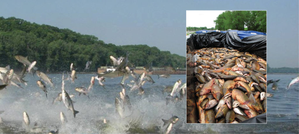
Figure 1. Asian carp jump out of the water in response to electrofishing. The Asian carp in the inset photograph were harvested from the Little Calumet River in Illinois in May, 2010, using rotenone, a toxin often used as an insecticide, in an effort to learn more about the population of the species. (credit main image: modification of work by USGS; credit inset: modification of work by Lt. David French, USCG)
This fish—actually a group of species including the silver, black, grass, and big head carp—has been farmed and eaten in China for over 1000 years. It is one of the most important aquaculture food resources worldwide. In the United States, however, Asian carp is considered a dangerous invasive species that disrupts community structure and composition to the point of threatening native species.
Learning Objectives
- Describe how ecologists measure population size and density
- Identify methods used to study population changes over time
- Describe how life history patterns are influenced by natural selection
- Explain the characteristics of and differences between exponential and logistic growth patterns
- Compare and contrast density-dependent growth regulation and density-independent growth regulation
- Compare and contrast K-selected and r-selected Species
- Discuss how the human population has changed over time
Population Demography
Populations are dynamic entities. Populations consist all of the species living within a specific area, and populations fluctuate based on a number of factors: seasonal and yearly changes in the environment, natural disasters such as forest fires and volcanic eruptions, and competition for resources between and within species. The statistical study of population dynamics, demography, uses a series of mathematical tools to investigate how populations respond to changes in their biotic and abiotic environments. Many of these tools were originally designed to study human populations. For example, life tables, which detail the life expectancy of individuals within a population, were initially developed by life insurance companies to set insurance rates. In fact, while the term “demographics” is commonly used when discussing humans, all living populations can be studied using this approach.
Population Size and Density
The study of any population usually begins by determining how many individuals of a particular species exist, and how closely associated they are with each other. Within a particular habitat, a population can be characterized by its population size (N), the total number of individuals, and its population density, the number of individuals within a specific area or volume. Population size and density are the two main characteristics used to describe and understand populations. For example, populations with more individuals may be more stable than smaller populations based on their genetic variability, and thus their potential to adapt to the environment. Alternatively, a member of a population with low population density (more spread out in the habitat), might have more difficulty finding a mate to reproduce compared to a population of higher density. As is shown in the Figure 2 below, smaller organisms tend to be more densely distributed than larger organisms.
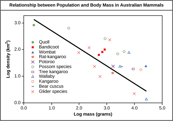
Figure 2. Australian mammals show a typical inverse relationship between population density and body size.
Practice Question
As this graph shows, population density typically decreases with increasing body size. Why do you think this is the case?
Population Research Methods
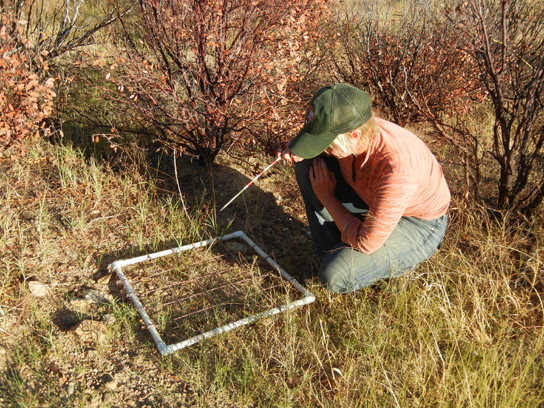
Figure 3. A scientist uses a quadrat to measure population size and density. (credit: NPS Sonoran Desert Network)
The most accurate way to determine population size is to simply count all of the individuals within the habitat. However, this method is often not logistically or economically feasible, especially when studying large habitats. Thus, scientists usually study populations by sampling a representative portion of each habitat and using this data to make inferences about the habitat as a whole. A variety of methods can be used to sample populations to determine their size and density. For immobile organisms such as plants, or for very small and slow-moving organisms, a quadrat may be used. A quadrat is a way of marking off square areas within a habitat, either by staking out an area with sticks and string, or by the use of a wood, plastic, or metal square placed on the ground. After setting the quadrats, researchers then count the number of individuals that lie within their boundaries. Multiple quadrat samples are performed throughout the habitat at several random locations. All of this data can then be used to estimate the population size and population density within the entire habitat. The number and size of quadrat samples depends on the type of organisms under study and other factors, including the density of the organism. For example, if sampling daffodils, a 1 m2 quadrat might be used whereas with giant redwoods, which are larger and live much further apart from each other, a larger quadrat of 100 m2 might be employed. This ensures that enough individuals of the species are counted to get an accurate sample that correlates with the habitat, including areas not sampled.
For mobile organisms, such as mammals, birds, or fish, a technique called mark and recapture is often used. This method involves marking a sample of captured animals in some way (such as tags, bands, paint, or other body markings), and then releasing them back into the environment to allow them to mix with the rest of the population; later, a new sample is collected, including some individuals that are marked (recaptures) and some individuals that are unmarked.
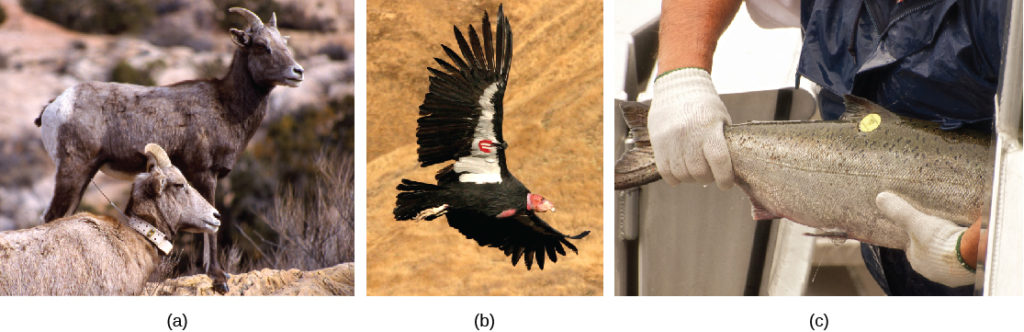
Figure 4. Mark and recapture is used to measure the population size of mobile animals such as (a) bighorn sheep, (b) the California condor, and (c) salmon. (credit a: modification of work by Neal Herbert, NPS; credit b: modification of work by Pacific Southwest Region USFWS; credit c: modification of work by Ingrid Taylar)
Using the ratio of marked and unmarked individuals, scientists determine how many individuals are in the sample. From this, calculations are used to estimate the total population size. This method assumes that the larger the population, the lower the percentage of tagged organisms that will be recaptured since they will have mixed with more untagged individuals. For example, if 80 deer are captured, tagged, and released into the forest, and later 100 deer are captured and 20 of them are already marked, we can determine the population size (N) using the following equation:
[latex]\displaystyle\frac{\text{number marked first catch}\times\text{total number of second catch}}{\text{number marked second catch}}=N[/latex]
Using our example, the population size would be estimated at 400:
[latex]\displaystyle\frac{80\times{100}}{20}=400[/latex]
Therefore, there are an estimated 400 total individuals in the original population.
There are some limitations to the mark and recapture method. Some animals from the first catch may learn to avoid capture in the second round, thus inflating population estimates. Alternatively, animals may preferentially be retrapped (especially if a food reward is offered), resulting in an underestimate of population size. Also, some species may be harmed by the marking technique, reducing their survival. A variety of other techniques have been developed, including the electronic tracking of animals tagged with radio transmitters and the use of data from commercial fishing and trapping operations to estimate the size and health of populations and communities.
Species Distribution
In addition to measuring simple density, further information about a population can be obtained by looking at the distribution of the individuals. Species dispersion patterns (or distribution patterns) show the spatial relationship between members of a population within a habitat at a particular point in time. In other words, they show whether members of the species live close together or far apart, and what patterns are evident when they are spaced apart.
Individuals in a population can be more or less equally spaced apart, dispersed randomly with no predictable pattern, or clustered in groups. These are known as uniform, random, and clumped dispersion patterns, respectively. Uniform dispersion is observed in plants that secrete substances inhibiting the growth of nearby individuals (such as the release of toxic chemicals by the sage plantSalvia leucophylla, a phenomenon called allelopathy) and in animals like the penguin that maintain a defined territory. An example of random dispersion occurs with dandelion and other plants that have wind-dispersed seeds that germinate wherever they happen to fall in a favorable environment. A clumped dispersion may be seen in plants that drop their seeds straight to the ground, such as oak trees, or animals that live in groups (schools of fish or herds of elephants). Clumped dispersions may also be a function of habitat heterogeneity. Thus, the dispersion of the individuals within a population provides more information about how they interact with each other than does a simple density measurement. Just as lower density species might have more difficulty finding a mate, solitary species with a random distribution might have a similar difficulty when compared to social species clumped together in groups.
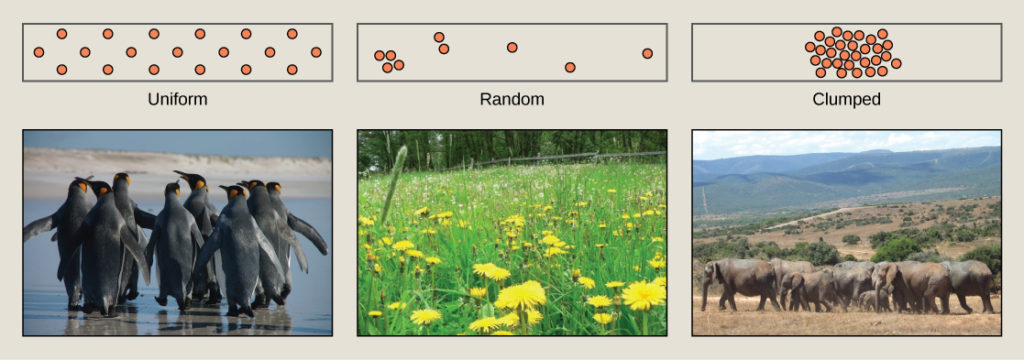
Figure 5. Species may have uniform, random, or clumped distribution. Territorial birds such as penguins tend to have uniform distribution. Plants such as dandelions with wind-dispersed seeds tend to be randomly distributed. Animals such as elephants that travel in groups exhibit clumped distribution. (credit a: modification of work by Ben Tubby; credit b: modification of work by Rosendahl; credit c: modification of work by Rebecca Wood)
Demography
While population size and density describe a population at one particular point in time, scientists must use demography to study the dynamics of a population. Demography is the statistical study of population changes over time: birth rates, death rates, and life expectancies. Each of these measures, especially birth rates, may be affected by the population characteristics described above. For example, a large population size results in a higher birth rate because more potentially reproductive individuals are present. In contrast, a large population size can also result in a higher death rate because of competition, disease, and the accumulation of waste. Similarly, a higher population density or a clumped dispersion pattern results in more potential reproductive encounters between individuals, which can increase birth rate. Lastly, a female-biased sex ratio (the ratio of males to females) or age structure (the proportion of population members at specific age ranges) composed of many individuals of reproductive age can increase birth rates.
In addition, the demographic characteristics of a population can influence how the population grows or declines over time. If birth and death rates are equal, the population remains stable. However, the population size will increase if birth rates exceed death rates; the population will decrease if birth rates are less than death rates. Life expectancy is another important factor; the length of time individuals remain in the population impacts local resources, reproduction, and the overall health of the population. These demographic characteristics are often displayed in the form of a life table.
Life Tables
Life tables provide important information about the life history of an organism. Life tables divide the population into age groups and often sexes, and show how long a member of that group is likely to live. They are modeled after actuarial tables used by the insurance industry for estimating human life expectancy. Life tables may include the probability of individuals dying before their next birthday (i.e., their mortality rate), the percentage of surviving individuals dying at a particular age interval, and their life expectancy at each interval. An example of a life table is shown in Table 1 from a study of Dall mountain sheep, a species native to northwestern North America. Notice that the population is divided into age intervals (column A). The mortality rate (per 1000), shown in column D, is based on the number of individuals dying during the age interval (column B) divided by the number of individuals surviving at the beginning of the interval (Column C), multiplied by 1000.
[latex]\displaystyle\text{mortality rate}=\frac{\text{number of individuals dying}}{\text{number of individuals surviving}}\times{N}[/latex]
For example, between ages three and four, 12 individuals die out of the 776 that were remaining from the original 1000 sheep. This number is then multiplied by 1000 to get the mortality rate per thousand.
[latex]\displaystyle\text{mortality rate}=\frac{12}{776}\times{1000}\approx{15.5}[/latex]
As can be seen from the mortality rate data (column D), a high death rate occurred when the sheep were between 6 and 12 months old, and then increased even more from 8 to 12 years old, after which there were few survivors. The data indicate that if a sheep in this population were to survive to age one, it could be expected to live another 7.7 years on average, as shown by the life expectancy numbers in column E.
| Table 1. Life Table of Dall Mountain Sheep[1] | ||||
|---|---|---|---|---|
| Age interval (years) | Number dying in age interval out of 1000 born | Number surviving at beginning of age interval out of 1000 born | Mortality rate per 1000 alive at beginning of age interval | Life expectancy or mean lifetime remaining to those attaining age interval |
| 0–0.5 | 54 | 1000 | 54.0 | 7.06 |
| 0.5–1 | 145 | 946 | 153.3 | — |
| 1–2 | 12 | 801 | 15.0 | 7.7 |
| 2–3 | 13 | 789 | 16.5 | 6.8 |
| 3–4 | 12 | 776 | 15.5 | 5.9 |
| 4–5 | 30 | 764 | 39.3 | 5.0 |
| 5–6 | 46 | 734 | 62.7 | 4.2 |
| 6–7 | 48 | 688 | 69.8 | 3.4 |
| 7–8 | 69 | 640 | 107.8 | 2.6 |
| 8–9 | 132 | 571 | 231.2 | 1.9 |
| 9–10 | 187 | 439 | 426.0 | 1.3 |
| 10–11 | 156 | 252 | 619.0 | 0.9 |
| 11–12 | 90 | 96 | 937.5 | 0.6 |
| 12–13 | 3 | 6 | 500.0 | 1.2 |
| 13–14 | 3 | 3 | 1000 | 0.7 |
Survivorship Curves
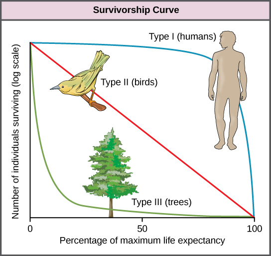
Figure 6. Survivorship curves show the distribution of individuals in a population according to age. Humans and most mammals have a Type I survivorship curve because death primarily occurs in the older years. Birds have a Type II survivorship curve, as death at any age is equally probable. Trees have a Type III survivorship curve because very few survive the younger years, but after a certain age, individuals are much more likely to survive.
Another tool used by population ecologists is a survivorship curve, which is a graph of the number of individuals surviving at each age interval plotted versus time (usually with data compiled from a life table). These curves allow us to compare the life histories of different populations. Humans and most primates exhibit a Type I survivorship curve because a high percentage of offspring survive their early and middle years—death occurs predominantly in older individuals. These types of species usually have small numbers of offspring at one time, and they give a high amount of parental care to them to ensure their survival. Birds are an example of an intermediate or Type II survivorship curve because birds die more or less equally at each age interval. These organisms also may have relatively few offspring and provide significant parental care. Trees, marine invertebrates, and most fishes exhibit a Type III survivorship curve because very few of these organisms survive their younger years; however, those that make it to an old age are more likely to survive for a relatively long period of time. Organisms in this category usually have a very large number of offspring, but once they are born, little parental care is provided. Thus these offspring are “on their own” and vulnerable to predation, but their sheer numbers assure the survival of enough individuals to perpetuate the species.
Life Histories and Natural Selection
A species’ life history describes the series of events over its lifetime, such as how resources are allocated for growth, maintenance, and reproduction. Life history traits affect the life table of an organism. A species’ life history is genetically determined and shaped by the environment and natural selection.
Life History Patterns and Energy Budgets
Energy is required by all living organisms for their growth, maintenance, and reproduction; at the same time, energy is often a major limiting factor in determining an organism’s survival. Plants, for example, acquire energy from the sun via photosynthesis, but must expend this energy to grow, maintain health, and produce energy-rich seeds to produce the next generation. Animals have the additional burden of using some of their energy reserves to acquire food. Furthermore, some animals must expend energy caring for their offspring. Thus, all species have an energy budget: they must balance energy intake with their use of energy for metabolism, reproduction, parental care, and energy storage (such as bears building up body fat for winter hibernation).
Parental Care and Fecundity
Fecundity is the potential reproductive capacity of an individual within a population. In other words, fecundity describes how many offspring could ideally be produced if an individual has as many offspring as possible, repeating the reproductive cycle as soon as possible after the birth of the offspring. In animals, fecundity is inversely related to the amount of parental care given to an individual offspring. Species, such as many marine invertebrates, that produce many offspring usually provide little if any care for the offspring (they would not have the energy or the ability to do so anyway). Most of their energy budget is used to produce many tiny offspring. Animals with this strategy are often self-sufficient at a very early age. This is because of the energy tradeoff these organisms have made to maximize their evolutionary fitness. Because their energy is used for producing offspring instead of parental care, it makes sense that these offspring have some ability to be able to move within their environment and find food and perhaps shelter. Even with these abilities, their small size makes them extremely vulnerable to predation, so the production of many offspring allows enough of them to survive to maintain the species.
Animal species that have few offspring during a reproductive event usually give extensive parental care, devoting much of their energy budget to these activities, sometimes at the expense of their own health. This is the case with many mammals, such as humans, kangaroos, and pandas. The offspring of these species are relatively helpless at birth and need to develop before they achieve self-sufficiency.
Plants with low fecundity produce few energy-rich seeds (such as coconuts and chestnuts) with each having a good chance to germinate into a new organism; plants with high fecundity usually have many small, energy-poor seeds (like orchids) that have a relatively poor chance of surviving. Although it may seem that coconuts and chestnuts have a better chance of surviving, the energy tradeoff of the orchid is also very effective. It is a matter of where the energy is used, for large numbers of seeds or for fewer seeds with more energy.
Early versus Late Reproduction
The timing of reproduction in a life history also affects species survival. Organisms that reproduce at an early age have a greater chance of producing offspring, but this is usually at the expense of their growth and the maintenance of their health. Conversely, organisms that start reproducing later in life often have greater fecundity or are better able to provide parental care, but they risk that they will not survive to reproductive age. Examples of this can be seen in fishes. Small fish like guppies use their energy to reproduce rapidly, but never attain the size that would give them defense against some predators. Larger fish, like the bluegill or shark, use their energy to attain a large size, but do so with the risk that they will die before they can reproduce or at least reproduce to their maximum. These different energy strategies and tradeoffs are key to understanding the evolution of each species as it maximizes its fitness and fills its niche. In terms of energy budgeting, some species “blow it all” and use up most of their energy reserves to reproduce early before they die. Other species delay having reproduction to become stronger, more experienced individuals and to make sure that they are strong enough to provide parental care if necessary.
Single versus Multiple Reproductive Events
Some life history traits, such as fecundity, timing of reproduction, and parental care, can be grouped together into general strategies that are used by multiple species. Semelparity occurs when a species reproduces only once during its lifetime and then dies. Such species use most of their resource budget during a single reproductive event, sacrificing their health to the point that they do not survive. Examples of semelparity are bamboo, which flowers once and then dies, and the Chinook salmon (Figure 7a), which uses most of its energy reserves to migrate from the ocean to its freshwater nesting area, where it reproduces and then dies. Scientists have posited alternate explanations for the evolutionary advantage of the Chinook’s post-reproduction death: a programmed suicide caused by a massive release of corticosteroid hormones, presumably so the parents can become food for the offspring, or simple exhaustion caused by the energy demands of reproduction; these are still being debated.
Iteroparity describes species that reproduce repeatedly during their lives. Some animals are able to mate only once per year, but survive multiple mating seasons. The pronghorn antelope is an example of an animal that goes into a seasonal estrus cycle (“heat”): a hormonally induced physiological condition preparing the body for successful mating (Figure 7b). Females of these species mate only during the estrus phase of the cycle. A different pattern is observed in primates, including humans and chimpanzees, which may attempt reproduction at any time during their reproductive years, even though their menstrual cycles make pregnancy likely only a few days per month during ovulation (Figure 7c).
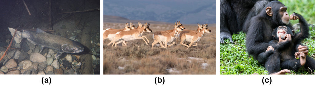
Figure 7. The (a) Chinook salmon mates once and dies. The (b) pronghorn antelope mates during specific times of the year during its reproductive life. Primates, such as humans and (c) chimpanzees, may mate on any day, independent of ovulation. (credit a: modification of work by Roger Tabor, USFWS; credit b: modification of work by Mark Gocke, USDA; credit c: modification of work by “Shiny Things”/Flickr)
Energy Budgets, Reproductive Costs, and Sexual Selection in Drosophila
Research into how animals allocate their energy resources for growth, maintenance, and reproduction has used a variety of experimental animal models. Some of this work has been done using the common fruit fly, Drosophila melanogaster. Studies have shown that not only does reproduction have a cost as far as how long male fruit flies live, but also fruit flies that have already mated several times have limited sperm remaining for reproduction. Fruit flies maximize their last chances at reproduction by selecting optimal mates.
In a 1981 study, male fruit flies were placed in enclosures with either virgin or inseminated females. The males that mated with virgin females had shorter life spans than those in contact with the same number of inseminated females with which they were unable to mate. This effect occurred regardless of how large (indicative of their age) the males were. Thus, males that did not mate lived longer, allowing them more opportunities to find mates in the future.
More recent studies, performed in 2006, show how males select the female with which they will mate and how this is affected by previous matings (Table 2).[2] Males were allowed to select between smaller and larger females. Findings showed that larger females had greater fecundity, producing twice as many offspring per mating as the smaller females did. Males that had previously mated, and thus had lower supplies of sperm, were termed “resource-depleted,” while males that had not mated were termed “non-resource-depleted.” The study showed that although non-resource-depleted males preferentially mated with larger females, this selection of partners was more pronounced in the resource-depleted males. Thus, males with depleted sperm supplies, which were limited in the number of times that they could mate before they replenished their sperm supply, selected larger, more fecund females, thus maximizing their chances for offspring. This study was one of the first to show that the physiological state of the male affected its mating behavior in a way that clearly maximizes its use of limited reproductive resources.
| Table 2 | |
|---|---|
| Ratio large/small females mated | |
| Non sperm-depleted | 8 ± 5 |
| Sperm-depleted | 15 ± 5 |
Male fruit flies that had previously mated (sperm-depleted) picked larger, more fecund females more often than those that had not mated (non-sperm-depleted). This change in behavior causes an increase in the efficiency of a limited reproductive resource: sperm.
These studies demonstrate two ways in which the energy budget is a factor in reproduction. First, energy expended on mating may reduce an animal’s lifespan, but by this time they have already reproduced, so in the context of natural selection this early death is not of much evolutionary importance. Second, when resources such as sperm (and the energy needed to replenish it) are low, an organism’s behavior can change to give them the best chance of passing their genes on to the next generation. These changes in behavior, so important to evolution, are studied in a discipline known as behavioral biology, or ethology, at the interface between population biology and psychology.
IN SUMMARY: LIFE HISTORIES AND NATURAL SELECTION
All species have evolved a pattern of living, called a life history strategy, in which they partition energy for growth, maintenance, and reproduction. These patterns evolve through natural selection; they allow species to adapt to their environment to obtain the resources they need to successfully reproduce. There is an inverse relationship between fecundity and parental care. A species may reproduce early in life to ensure surviving to a reproductive age or reproduce later in life to become larger and healthier and better able to give parental care. A species may reproduce once (semelparity) or many times (iteroparity) in its life.
Environmental Limits to Population Growth
Although life histories describe the way many characteristics of a population (such as their age structure) change over time in a general way, population ecologists make use of a variety of methods to model population dynamics mathematically. These more precise models can then be used to accurately describe changes occurring in a population and better predict future changes. Certain models that have been accepted for decades are now being modified or even abandoned due to their lack of predictive ability, and scholars strive to create effective new models.
Exponential Growth
Charles Darwin, in his theory of natural selection, was greatly influenced by the English clergyman Thomas Malthus. Malthus published a book in 1798 stating that populations with unlimited natural resources grow very rapidly, and then population growth decreases as resources become depleted. This accelerating pattern of increasing population size is called exponential growth.
The best example of exponential growth is seen in bacteria. Bacteria are prokaryotes that reproduce by prokaryotic fission. This division takes about an hour for many bacterial species. If 1000 bacteria are placed in a large flask with an unlimited supply of nutrients (so the nutrients will not become depleted), after an hour, there is one round of division and each organism divides, resulting in 2000 organisms—an increase of 1000. In another hour, each of the 2000 organisms will double, producing 4000, an increase of 2000 organisms. After the third hour, there should be 8000 bacteria in the flask, an increase of 4000 organisms. The important concept of exponential growth is that the population growth rate—the number of organisms added in each reproductive generation—is accelerating; that is, it is increasing at a greater and greater rate. After 1 day and 24 of these cycles, the population would have increased from 1000 to more than 16 billion. When the population size, N, is plotted over time, a J-shaped growth curve is produced (Figure 8).
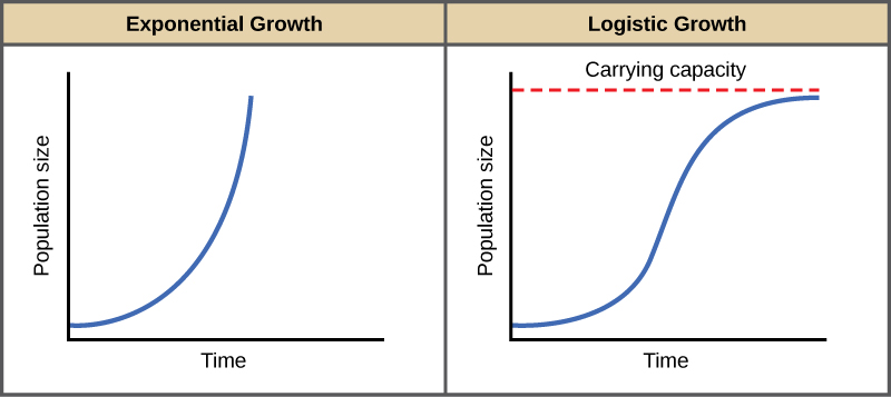
Figure 8. When resources are unlimited, populations exhibit exponential growth, resulting in a J-shaped curve. When resources are limited, populations exhibit logistic growth. In logistic growth, population expansion decreases as resources become scarce, and it levels off when the carrying capacity of the environment is reached, resulting in an S-shaped curve.
The bacteria example is not representative of the real world where resources are limited. Furthermore, some bacteria will die during the experiment and thus not reproduce, lowering the growth rate. Therefore, when calculating the growth rate of a population, the death rate (D) (number organisms that die during a particular time interval) is subtracted from the birth rate (B) (number organisms that are born during that interval). This is shown in the following formula:
[latex]\displaystyle\frac{\Delta{N}\left(\text{change in number}\right)}{\Delta{T}\left(\text{change in time}\right)}=B\left(\text{birth rate}\right)-D\left(\text{death rate}\right)[/latex]
The birth rate is usually expressed on a per capita (for each individual) basis. Thus, B (birth rate) = bN (the per capita birth rate “b” multiplied by the number of individuals “N”) and D (death rate) =dN (the per capita death rate “d” multiplied by the number of individuals “N”). Additionally, ecologists are interested in the population at a particular point in time, an infinitely small time interval. For this reason, the terminology of differential calculus is used to obtain the “instantaneous” growth rate, replacing the change in number and time with an instant-specific measurement of number and time.
[latex]\frac{dN}{dT}=bN=dN=\left(b-d\right)N[/latex]
Notice that the “d” associated with the first term refers to the derivative (as the term is used in calculus) and is different from the death rate, also called “d.” The difference between birth and death rates is further simplified by substituting the term “r” (intrinsic rate of increase) for the relationship between birth and death rates:
[latex]\frac{dN}{dT}=rN[/latex]
The value “r” can be positive, meaning the population is increasing in size; or negative, meaning the population is decreasing in size; or zero, where the population’s size is unchanging, a condition known as zero population growth. A further refinement of the formula recognizes that different species have inherent differences in their intrinsic rate of increase (often thought of as the potential for reproduction), even under ideal conditions. Obviously, a bacterium can reproduce more rapidly and have a higher intrinsic rate of growth than a human. The maximal growth rate for a species is its biotic potential, or rmax, thus changing the equation to:
[latex]\frac{dN}{dT}=r_{\text{max}}N[/latex]
Logistic Growth
Exponential growth is possible only when infinite natural resources are available; this is not the case in the real world. Charles Darwin recognized this fact in his description of the “struggle for existence,” which states that individuals will compete (with members of their own or other species) for limited resources. The successful ones will survive to pass on their own characteristics and traits (which we know now are transferred by genes) to the next generation at a greater rate (natural selection). To model the reality of limited resources, population ecologists developed the logistic growth model.
Carrying Capacity and the Logistic Model
In the real world, with its limited resources, exponential growth cannot continue indefinitely. Exponential growth may occur in environments where there are few individuals and plentiful resources, but when the number of individuals gets large enough, resources will be depleted, slowing the growth rate. Eventually, the growth rate will plateau or level off (Figure 8). This population size, which represents the maximum population size that a particular environment can support, is called the carrying capacity, orK.
The formula we use to calculate logistic growth adds the carrying capacity as a moderating force in the growth rate. The expression “K – N” is indicative of how many individuals may be added to a population at a given stage, and “K – N” divided by “K” is the fraction of the carrying capacity available for further growth. Thus, the exponential growth model is restricted by this factor to generate the logistic growth equation:
[latex]\displaystyle\frac{dN}{dT}=r_{\text{max}}\frac{dN}{dT}=r_{\text{max}}N\frac{\left(K-N\right)}{K}[/latex]
Notice that when N is very small, (K-N)/K becomes close to K/K or 1, and the right side of the equation reduces to rmaxN, which means the population is growing exponentially and is not influenced by carrying capacity. On the other hand, when N is large, (K-N)/K come close to zero, which means that population growth will be slowed greatly or even stopped. Thus, population growth is greatly slowed in large populations by the carrying capacity K. This model also allows for the population of a negative population growth, or a population decline. This occurs when the number of individuals in the population exceeds the carrying capacity (because the value of (K-N)/K is negative).
A graph of this equation yields an S-shaped curve (Figure 8), and it is a more realistic model of population growth than exponential growth. There are three different sections to an S-shaped curve. Initially, growth is exponential because there are few individuals and ample resources available. Then, as resources begin to become limited, the growth rate decreases. Finally, growth levels off at the carrying capacity of the environment, with little change in population size over time.
Role of Intraspecific Competition
The logistic model assumes that every individual within a population will have equal access to resources and, thus, an equal chance for survival. For plants, the amount of water, sunlight, nutrients, and the space to grow are the important resources, whereas in animals, important resources include food, water, shelter, nesting space, and mates.
In the real world, phenotypic variation among individuals within a population means that some individuals will be better adapted to their environment than others. The resulting competition between population members of the same species for resources is termed intraspecific competition (intra– = “within”; –specific = “species”). Intraspecific competition for resources may not affect populations that are well below their carrying capacity—resources are plentiful and all individuals can obtain what they need. However, as population size increases, this competition intensifies. In addition, the accumulation of waste products can reduce an environment’s carrying capacity.
Examples of Logistic Growth
Yeast, a microscopic fungus used to make bread and alcoholic beverages, exhibits the classical S-shaped curve when grown in a test tube (Figure 9). Its growth levels off as the population depletes the nutrients that are necessary for its growth. In the real world, however, there are variations to this idealized curve.
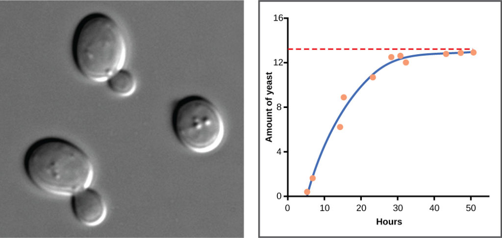
Figure 9. Yeast grown in ideal conditions in a test tube show a classical S-shaped logistic growth curve.
Examples in wild populations include sheep and harbor seals (Figure 10). In both examples, the population size exceeds the carrying capacity for short periods of time and then falls below the carrying capacity afterwards. This fluctuation in population size continues to occur as the population oscillates around its carrying capacity. Still, even with this oscillation, the logistic model is confirmed.
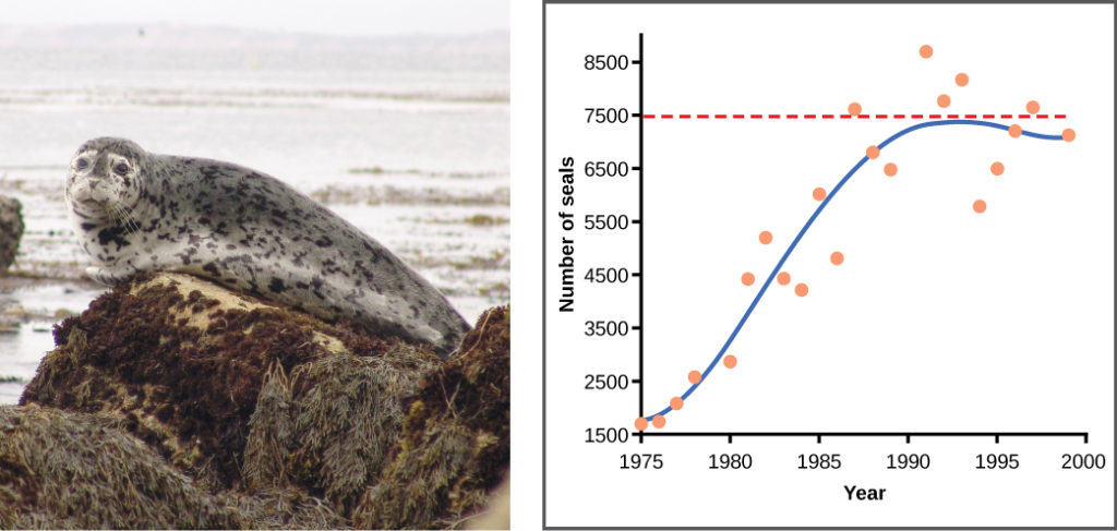
Figure 10. A natural population of seals shows real-world fluctuation.
Practice Question
If the major food source of the seals declines due to pollution or overfishing, which of the following would likely occur?
- The carrying capacity of seals would decrease, as would the seal population.
- The carrying capacity of seals would decrease, but the seal population would remain the same.
- The number of seal deaths would increase but the number of births would also increase, so the population size would remain the same.
- The carrying capacity of seals would remain the same, but the population of seals would decrease.
IN SUMMARY: Environmental Limits to Population Growth
Populations with unlimited resources grow exponentially, with an accelerating growth rate. When resources become limiting, populations follow a logistic growth curve. The population of a species will level off at the carrying capacity of its environment.
Population Dynamics and Regulation
The logistic model of population growth, while valid in many natural populations and a useful model, is a simplification of real-world population dynamics. Implicit in the model is that the carrying capacity of the environment does not change, which is not the case. The carrying capacity varies annually: for example, some summers are hot and dry whereas others are cold and wet. In many areas, the carrying capacity during the winter is much lower than it is during the summer. Also, natural events such as earthquakes, volcanoes, and fires can alter an environment and hence its carrying capacity. Additionally, populations do not usually exist in isolation. They engage in interspecific competition: that is, they share the environment with other species, competing with them for the same resources. These factors are also important to understanding how a specific population will grow.
Nature regulates population growth in a variety of ways. These are grouped into density-dependent factors, in which the density of the population at a given time affects growth rate and mortality, and density-independent factors, which influence mortality in a population regardless of population density. Note that in the former, the effect of the factor on the population depends on the density of the population at onset. Conservation biologists want to understand both types because this helps them manage populations and prevent extinction or overpopulation.
Density-dependent Regulation
Most density-dependent factors are biological in nature (biotic), and include predation, inter- and intraspecific competition, accumulation of waste, and diseases such as those caused by parasites. Usually, the denser a population is, the greater its mortality rate. For example, during intra- and interspecific competition, the reproductive rates of the individuals will usually be lower, reducing their population’s rate of growth. In addition, low prey density increases the mortality of its predator because it has more difficulty locating its food source.
An example of density-dependent regulation is shown in Figure 11 with results from a study focusing on the giant intestinal roundworm (Ascaris lumbricoides), a parasite of humans and other mammals.[3] Denser populations of the parasite exhibited lower fecundity: they contained fewer eggs. One possible explanation for this is that females would be smaller in more dense populations (due to limited resources) and that smaller females would have fewer eggs. This hypothesis was tested and disproved in a 2009 study which showed that female weight had no influence.[4] The actual cause of the density-dependence of fecundity in this organism is still unclear and awaiting further investigation.[5]
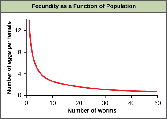
Figure 11. In this population of roundworms, fecundity (number of eggs) decreases with population density.
Density-independent Regulation and Interaction with Density-dependent Factors
Many factors, typically physical or chemical in nature (abiotic), influence the mortality of a population regardless of its density, including weather, natural disasters, and pollution. An individual deer may be killed in a forest fire regardless of how many deer happen to be in that area. Its chances of survival are the same whether the population density is high or low. The same holds true for cold winter weather.
In real-life situations, population regulation is very complicated and density-dependent and independent factors can interact. A dense population that is reduced in a density-independent manner by some environmental factor(s) will be able to recover differently than a sparse population. For example, a population of deer affected by a harsh winter will recover faster if there are more deer remaining to reproduce.
Why Did the Woolly Mammoth Go Extinct?
It’s easy to get lost in the discussion of dinosaurs and theories about why they went extinct 65 million years ago. Was it due to a meteor slamming into Earth near the coast of modern-day Mexico, or was it from some long-term weather cycle that is not yet understood? One hypothesis that will never be proposed is that humans had something to do with it. Mammals were small, insignificant creatures of the forest 65 million years ago, and no humans existed.
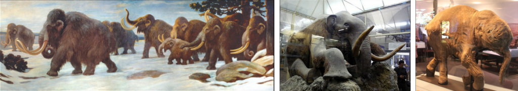
Figure 12. The three photos include: (a) 1916 mural of a mammoth herd from the American Museum of Natural History, (b) the only stuffed mammoth in the world, from the Museum of Zoology located in St. Petersburg, Russia, and (c) a one-month-old baby mammoth, named Lyuba, discovered in Siberia in 2007. (credit a: modification of work by Charles R. Knight; credit b: modification of work by “Tanapon”/Flickr; credit c: modification of work by Matt Howry)
Woolly mammoths, however, began to go extinct about 10,000 years ago, when they shared the Earth with humans who were no different anatomically than humans today. Mammoths survived in isolated island populations as recently as 1700 BC. We know a lot about these animals from carcasses found frozen in the ice of Siberia and other regions of the north. Scientists have sequenced at least 50 percent of its genome and believe mammoths are between 98 and 99 percent identical to modern elephants.
It is commonly thought that climate change and human hunting led to their extinction. A 2008 study estimated that climate change reduced the mammoth’s range from 3,000,000 square miles 42,000 years ago to 310,000 square miles 6,000 years ago.[6] It is also well documented that humans hunted these animals. A 2012 study showed that no single factor was exclusively responsible for the extinction of these magnificent creatures.[7] In addition to human hunting, climate change, and reduction of habitat, these scientists demonstrated another important factor in the mammoth’s extinction was the migration of humans across the Bering Strait to North America during the last ice age 20,000 years ago.
Additionally, a 2017 study indicates the woolly mammoth genome began to accumulate excess defects as the population size collapsed to a mere 300 individuals living on an isolated island [8] The exact role this genomic “meltdown” may have played is unknown, but it did occur just prior to the extinction of this species.
The maintenance of stable populations was and is very complex, with many interacting factors determining the outcome. It is important to remember that humans are also part of nature. Once we contributed to a species’s decline using primitive hunting technology only.
Modern Theories of Life History
The r– and K-selection theory, although accepted for decades and used for much groundbreaking research, has now been reconsidered, and many population biologists have abandoned or modified it. Over the years, several studies attempted to confirm the theory, but these attempts have largely failed. Many species were identified that did not follow the theory’s predictions. Furthermore, the theory ignored the age-specific mortality of the populations which scientists now know is very important. New demographic-based models of life history evolution have been developed which incorporate many ecological concepts included in r– and K-selection theory as well as population age structure and mortality factors.
Life Histories of K-selected and r-selected Species
While reproductive strategies play a key role in life histories, they do not account for important factors like limited resources and competition. The regulation of population growth by these factors can be used to introduce a classical concept in population biology, that of K-selected versus r-selected species.
Early Theories about Life History
By the second half of the twentieth century, the concept of K- and r-selected species was used extensively and successfully to study populations. The concept relates not only reproductive strategies, but also to a species’ habitat and behavior, especially in the way that they obtain resources and care for their young. It includes length of life and survivorship factors as well. For this analysis, population biologists have grouped species into the two large categories—K-selected and r-selected—although they are really two ends of a continuum.
K-selected species are species selected by stable, predictable environments. Populations of K-selected species tend to exist close to their carrying capacity (hence the term K-selected) where intraspecific competition is high. These species have few, large offspring, a long gestation period, and often give long-term care to their offspring (Table 3). While larger in size when born, the offspring are relatively helpless and immature at birth. By the time they reach adulthood, they must develop skills to compete for natural resources. In plants, scientists think of parental care more broadly: how long fruit takes to develop or how long it remains on the plant are determining factors in the time to the next reproductive event. Examples of K-selected species are primates including humans), elephants, and plants such as oak trees (Figure 13).
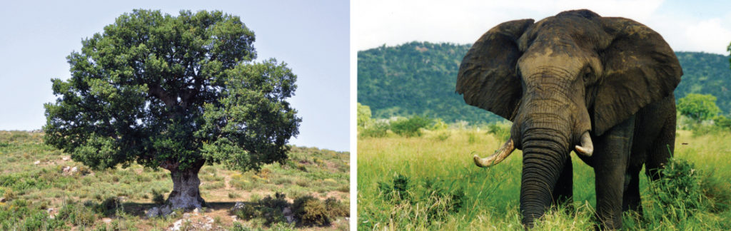
Figure 13. Elephants are considered K-selected species as they live long, mature late, and provide long-term parental care to few offspring. Oak trees produce many offspring that do not receive parental care, but are considered K-selected species based on longevity and late maturation.
Oak trees grow very slowly and take, on average, 20 years to produce their first seeds, known as acorns. As many as 50,000 acorns can be produced by an individual tree, but the germination rate is low as many of these rot or are eaten by animals such as squirrels. In some years, oaks may produce an exceptionally large number of acorns, and these years may be on a two- or three-year cycle depending on the species of oak (r-selection).
As oak trees grow to a large size and for many years before they begin to produce acorns, they devote a large percentage of their energy budget to growth and maintenance. The tree’s height and size allow it to dominate other plants in the competition for sunlight, the oak’s primary energy resource. Furthermore, when it does reproduce, the oak produces large, energy-rich seeds that use their energy reserve to become quickly established (K-selection).
In contrast, r-selected species have a large number of small offspring (hence their r designation). This strategy is often employed in unpredictable or changing environments. Animals that are r-selected do not give long-term parental care and the offspring are relatively mature and self-sufficient at birth. Examples of r-selected species are marine invertebrates, such as jellyfish, and plants, such as the dandelion (Figure 14). Dandelions have small seeds that are wind dispersed long distances. Many seeds are produced simultaneously to ensure that at least some of them reach a hospitable environment. Seeds that land in inhospitable environments have little chance for survival since their seeds are low in energy content. Note that survival is not necessarily a function of energy stored in the seed itself.
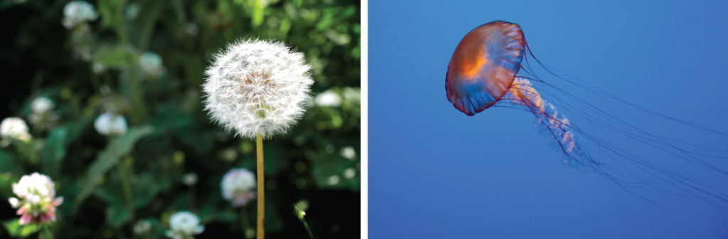
Figure 14. Dandelions and jellyfish are both considered r-selected species as they mature early, have short lifespans, and produce many offspring that receive no parental care.
| Table 3. Characteristics of K-selected and r-selected species | |
|---|---|
| Characteristics of K-selected species | Characteristics of r-selected species |
| Mature late | Mature early |
| Greater longevity | Lower longevity |
| Increased parental care | Decreased parental care |
| Increased competition | Decreased competition |
| Fewer offspring | More offspring |
| Larger offspring | Smaller offspring |
Human Population Growth
Concepts of animal population dynamics can be applied to human population growth. Humans are not unique in their ability to alter their environment. For example, beaver dams alter the stream environment where they are built. Humans, however, have the ability to alter their environment to increase its carrying capacity sometimes to the detriment of other species (e.g., via artificial selection for crops that have a higher yield). Earth’s human population is growing rapidly, to the extent that some worry about the ability of the earth’s environment to sustain this population, as long-term exponential growth carries the potential risks of famine, disease, and large-scale death.
Although humans have increased the carrying capacity of their environment, the technologies used to achieve this transformation have caused unprecedented changes to Earth’s environment, altering ecosystems to the point where some may be in danger of collapse. The depletion of the ozone layer, erosion due to acid rain, and damage from global climate change are caused by human activities. The ultimate effect of these changes on our carrying capacity is unknown. As some point out, it is likely that the negative effects of increasing carrying capacity will outweigh the positive ones—the carrying capacity of the world for human beings might actually decrease.
The world’s human population is currently experiencing exponential growth even though human reproduction is far below its biotic potential (Figure 15). To reach its biotic potential, all females would have to become pregnant every nine months or so during their reproductive years. Also, resources would have to be such that the environment would support such growth. Neither of these two conditions exists. In spite of this fact, human population is still growing exponentially.
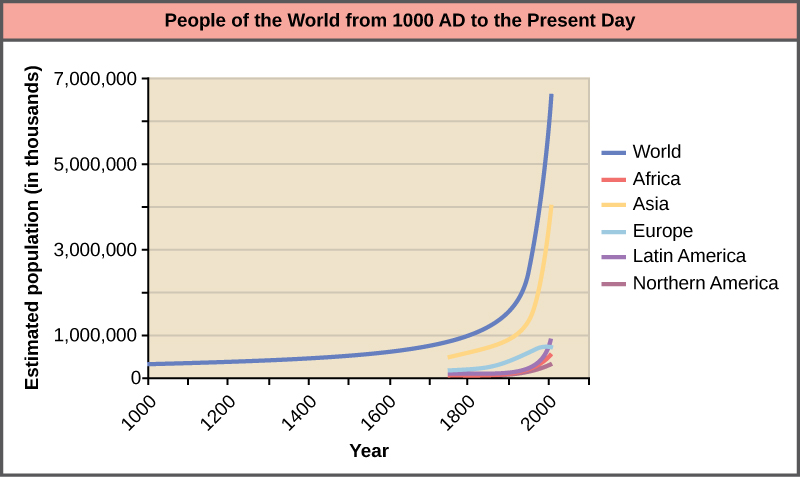
Figure 15. Human population growth since 1000 AD is exponential (dark blue line). Notice that while the population in Asia (yellow line), which has many economically underdeveloped countries, is increasing exponentially, the population in Europe (light blue line), where most of the countries are economically developed, is growing much more slowly.
A consequence of exponential human population growth is the time that it takes to add a particular number of humans to the Earth is becoming shorter. Figure 16 shows that 123 years were necessary to add 1 billion humans in 1930, but it only took 24 years to add two billion people between 1975 and 1999. As already discussed, at some point it would appear that our ability to increase our carrying capacity indefinitely on a finite world is uncertain. Without new technological advances, the human growth rate has been predicted to slow in the coming decades. However, the population will still be increasing and the threat of overpopulation remains.
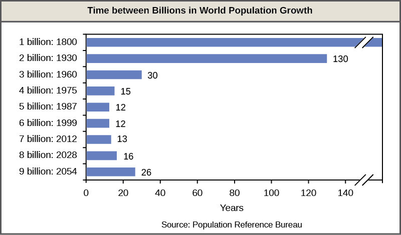
Figure 16. The time between the addition of each billion human beings to Earth decreases over time. (credit: modification of work by Ryan T. Cragun)
Overcoming Density-Dependent Regulation
Humans are unique in their ability to alter their environment with the conscious purpose of increasing its carrying capacity. This ability is a major factor responsible for human population growth and a way of overcoming density-dependent growth regulation. Much of this ability is related to human intelligence, society, and communication. Humans can construct shelter to protect them from the elements and have developed agriculture and domesticated animals to increase their food supplies. In addition, humans use language to communicate this technology to new generations, allowing them to improve upon previous accomplishments.
Other factors in human population growth are migration and public health. Humans originated in Africa, but have since migrated to nearly all inhabitable land on the Earth. Public health, sanitation, and the use of antibiotics and vaccines have decreased the ability of infectious disease to limit human population growth. In the past, diseases such as the bubonic plaque of the fourteenth century killed between 30 and 60 percent of Europe’s population and reduced the overall world population by as many as 100 million people. Today, the threat of infectious disease, while not gone, is certainly less severe. According to the World Health Organization, global death from infectious disease declined from 16.4 million in 1993 to 14.7 million in 1992. To compare to some of the epidemics of the past, the percentage of the world’s population killed between 1993 and 2002 decreased from 0.30 percent of the world’s population to 0.24 percent. Thus, it appears that the influence of infectious disease on human population growth is becoming less significant.
Age Structure, Population Growth, and Economic Development
The age structure of a population is an important factor in population dynamics. Age structure is the proportion of a population at different age ranges. Age structure allows better prediction of population growth, plus the ability to associate this growth with the level of economic development in the region. Countries with rapid growth have a pyramidal shape in their age structure diagrams, showing a preponderance of younger individuals, many of whom are of reproductive age or will be soon (Figure 17). This pattern is most often observed in underdeveloped countries where individuals do not live to old age because of less-than-optimal living conditions. Age structures of areas with slow growth, including developed countries such as the United States, still have a pyramidal structure, but with many fewer young and reproductive-aged individuals and a greater proportion of older individuals. Other developed countries, such as Italy, have zero population growth. The age structure of these populations is more conical, with an even greater percentage of middle-aged and older individuals. The actual growth rates in different countries are shown in Figure 18, with the highest rates tending to be in the less economically developed countries of Africa and Asia.
Practice Question
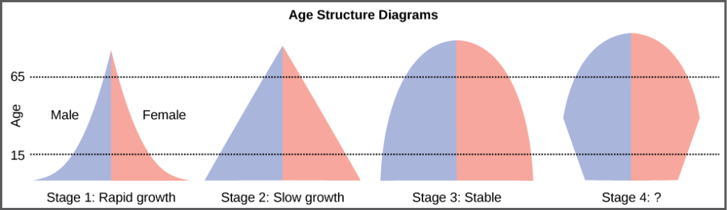
Figure 17. Typical age structure diagrams are shown. The rapid growth diagram narrows to a point, indicating that the number of individuals decreases rapidly with age. In the slow growth model, the number of individuals decreases steadily with age. Stable population diagrams are rounded on the top, showing that the number of individuals per age group decreases gradually, and then increases for the older part of the population.
Age structure diagrams for rapidly growing, slow growing and stable populations are shown in stages 1 through 3. What type of population change do you think stage 4 represents?
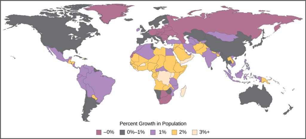
Figure 18. The percent growth rate of population in different countries is shown. Notice that the highest growth is occurring in less economically developed countries in Africa and Asia.
Long-Term Consequences of Exponential Human Population Growth
Many dire predictions have been made about the world’s population leading to a major crisis called the “population explosion.” In the 1968 book The Population Bomb, biologist Dr. Paul R. Ehrlich wrote, “The battle to feed all of humanity is over. In the 1970s hundreds of millions of people will starve to death in spite of any crash programs embarked upon now. At this late date nothing can prevent a substantial increase in the world death rate.” While many critics view this statement as an exaggeration, the laws of exponential population growth are still in effect, and unchecked human population growth cannot continue indefinitely.
Efforts to control population growth led to the one-child policy in China, which used to include more severe consequences, but now imposes fines on urban couples who have more than one child. Due to the fact that some couples wish to have a male heir, many Chinese couples continue to have more than one child. The policy itself, its social impacts, and the effectiveness of limiting overall population growth are controversial. In spite of population control policies, the human population continues to grow. At some point the food supply may run out because of the subsequent need to produce more and more food to feed our population. The United Nations estimates that future world population growth may vary from 6 billion (a decrease) to 16 billion people by the year 2100. There is no way to know whether human population growth will moderate to the point where the crisis described by Dr. Ehrlich will be averted.
Another result of population growth is the endangerment of the natural environment. Many countries have attempted to reduce the human impact on climate change by reducing their emission of the greenhouse gas carbon dioxide. However, these treaties have not been ratified by every country, and many underdeveloped countries trying to improve their economic condition may be less likely to agree with such provisions if it means slower economic development. Furthermore, the role of human activity in causing climate change has become a hotly debated socio-political issue in some developed countries, including the United States. Thus, we enter the future with considerable uncertainty about our ability to curb human population growth and protect our environment.
Video Review
The world’s human population is growing at an exponential rate. Humans have increased the world’s carrying capacity through migration, agriculture, medical advances, and communication. The age structure of a population allows us to predict population growth. Unchecked human population growth could have dire long-term effects on our environment.
This video tells us the specifics of why and how human population growth has happened over the past hundred and fifty years or so, and how those specifics relate to ecology.
Check Your Understanding
Answer the question(s) below to see how well you understand the topics covered in the previous section. This short quiz does not count toward your grade in the class, and you can retake it an unlimited number of times.
Use this quiz to check your understanding and decide whether to (1) study the previous section further or (2) move on to the next section.
Candela Citations
- Introduction to Population Ecology. Authored by: Shelli Carter and Lumen Learning. Provided by: Lumen Learning. License: CC BY: Attribution
- Biology. Provided by: OpenStax CNX. Located at: http://cnx.org/contents/185cbf87-c72e-48f5-b51e-f14f21b5eabd@10.8. License: CC BY: Attribution. License Terms: Download for free at http://cnx.org/contents/185cbf87-c72e-48f5-b51e-f14f21b5eabd@10.8
- Human Population Growth. Authored by: CrashCourse. Located at: https://youtu.be/E8dkWQVFAoA. License: All Rights Reserved. License Terms: Standard YouTube License
- Data Adapted from Edward S. Deevey, Jr., “Life Tables for Natural Populations of Animals,” The Quarterly Review of Biology 22, no. 4 (December 1947): 283–314. ↵
- Adapted from Phillip G. Byrne and William R. Rice, “Evidence for adaptive male mate choice in the fruit fly Drosophila melanogaster,” Proc Biol Sci. 273, no. 1589 (2006): 917–922, doi: 10.1098/rspb.2005.3372. ↵
- N.A. Croll et al., “The Population Biology and Control of Ascaris lumbricoides in a Rural Community in Iran.” Transactions of the Royal Society of Tropical Medicine and Hygiene 76, no. 2 (1982): 187-197, doi:10.1016/0035-9203(82)90272-3. ↵
- Martin Walker et al., “Density-Dependent Effects on the Weight of Female Ascaris lumbricoides Infections of Humans and its Impact on Patterns of Egg Production.” Parasites & Vectors 2, no. 11 (February 2009), doi:10.1186/1756-3305-2-11. ↵
- N.A. Croll et al., “The Population Biology and Control of Ascaris lumbricoides in a Rural Community in Iran.” Transactions of the Royal Society of Tropical Medicine and Hygiene 76, no. 2 (1982): 187-197, doi:10.1016/0035-9203(82)90272-3. ↵
- David Nogués-Bravo et al., “Climate Change, Humans, and the Extinction of the Woolly Mammoth.” PLoS Biol 6 (April 2008): e79, doi:10.1371/journal.pbio.0060079. ↵
- G.M. MacDonald et al., “Pattern of Extinction of the Woolly Mammoth in Beringia.” Nature Communications 3, no. 893 (June 2012), doi:10.1038/ncomms1881. ↵
- Rogers, R.L, and Slatkin, M., "Excess of genomic defects in a woolly mammoth on Wrangel island." PLoS Genetics 13(3) (2017): e1006601, doi:10.1371/journal.pgen.1006601. ↵