Learning Objectives
- Draw conclusions about a difference in population proportions from a simulation.
The Sampling Distribution of Differences in Sample Proportions
Let’s summarize what we have observed about the sampling distribution of the differences in sample proportions. We want to create a mathematical model of the sampling distribution, so we need to understand when we can use a normal curve. We also need to understand how the center and spread of the sampling distribution relates to the population proportions.
Shape:
In each situation we have encountered so far, the distribution of differences between sample proportions appears somewhat normal, but that is not always true. We discuss conditions for use of a normal model later.
Center:
Regardless of shape, the mean of the distribution of sample differences is the difference between the population proportions, p1 – p2. This is always true if we look at the long-run behavior of the differences in sample proportions.
Spread:
We have observed that larger samples have less variability. Advanced theory gives us this formula for the standard error in the distribution of differences between sample proportions:
[latex]\sqrt{\frac{{p}_{1}(1-{p}_{1})}{{n}_{1}}+\frac{{p}_{2}(1-{p}_{2})}{{n}_{2}}}[/latex]
Notice the following:
- The terms under the square root are familiar. These terms are used to compute the standard errors for the individual sampling distributions of [latex]{\stackrel{ˆ}{p}}_{1}[/latex] and [latex]{\stackrel{ˆ}{p}}_{2}[/latex] .
- The sample size is in the denominator of each term. As we learned earlier this means that increases in sample size result in a smaller standard error.
Comment
Let’s look at the relationship between the sampling distribution of differences between sample proportions and the sampling distributions for the individual sample proportions we studied in Linking Probability to Statistical Inference. We compare these distributions in the following table.
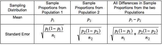
Notice the relationship between the means:
- The mean of the differences is the difference of the means. This makes sense. The mean of each sampling distribution of individual proportions is the population proportion, so the mean of the sampling distribution of differences is the difference in population proportions.
Notice the relationship between standard errors:
- The standard error of differences relates to the standard errors of the sampling distributions for individual proportions. Look at the terms under the square roots. Since we add these terms, the standard error of differences is always larger than the standard error in the sampling distributions of individual proportions. In other words, there is more variability in the differences.
Variability and Variance
In this module, we sample from two populations of categorical data, and compute sample proportions from each.
We have seen that the means of the sampling distributions of sample proportions are [latex]{p}_{1}\text{}\mathrm{and}\text{}{p}_{2}[/latex] and the standard errors are [latex]\sqrt{\frac{{p}_{1}(1-{p}_{1})}{{n}_{1}}}\text{}\mathrm{and}\text{}\sqrt{\frac{{p}_{2}(1-{p}_{2})}{{n}_{2}}}[/latex] .
Statisticians often refer to the square of a standard deviation or standard error as a variance. The variances of the sampling distributions of sample proportion are
[latex]\frac{{p}_{1}(1-{p}_{1})}{{n}_{1}}\text{}\mathrm{and}\text{}\frac{{p}_{2}(1-{p}_{2})}{{n}_{2}}[/latex]
If we add these variances we get the variance of the differences between sample proportions.
[latex]\frac{{p}_{1}(1-{p}_{1})}{{n}_{1}}\text{}+\text{}\frac{{p}_{2}(1-{p}_{2})}{{n}_{2}}[/latex]
For the sampling distribution of all differences, [latex]{\stackrel{ˆ}{p}}_{1}-{\stackrel{ˆ}{p}}_{2}[/latex] the mean, [latex]\mathrm{μ}{\stackrel{ˆ}{p}}_{1}-{\stackrel{ˆ}{p}}_{2}[/latex] , of all differences is the difference of the means [latex]{p}_{1}-{p}_{2}[/latex] . The variance of all differences, [latex]{\mathrm{σ}}^{2}{\stackrel{ˆ}{p}}_{1}-{\stackrel{ˆ}{p}}_{2}[/latex] , is the sum of the variances, [latex]\frac{{p}_{1}(1-{p}_{1})}{{n}_{1}}\text{}+\text{}\frac{{p}_{2}(1-{p}_{2})}{{n}_{2}}[/latex] .
We will now do some problems similar to problems we did earlier. Only now, we do not use a simulation to make observations about the variability in the differences of sample proportions. Instead, we use the mean and standard error of the sampling distribution. But our reasoning is the same.
Example
Controversy about HPV Vaccine
During a debate between Republican presidential candidates in 2011, Michele Bachmann, one of the candidates, implied that the vaccine for HPV is unsafe for children and can cause mental retardation. Scientists and other healthcare professionals immediately produced evidence to refute this claim. A USA Today article, “No Evidence HPV Vaccines Are Dangerous” (September 19, 2011), described two studies by the Centers for Disease Control and Prevention (CDC) that track the safety of the vaccine. Here is an excerpt from the article:
- First, the CDC monitors reports to the Vaccine Adverse Event Reporting System, a database to which anyone can report a suspected side effect. CDC officials then investigate to see whether reported problems could possibly be caused by vaccines or are simply a coincidence. Second, the CDC has been following girls who receive the vaccine over time, comparing them with a control group of unvaccinated girls….Again, the HPV vaccine has been found to be safe.
According to an article by Elizabeth Rosenthal, “Drug Makers’ Push Leads to Cancer Vaccines’ Rise” (New York Times, August 19, 2008), the FDA and CDC said that “with millions of vaccinations, by chance alone some serious adverse effects and deaths will occur in the time period following vaccination, but have nothing to do with the vaccine.” The article stated that the FDA and CDC monitor data to determine if more serious effects occur than would be expected from chance alone.
According to another source, the CDC data suggests that serious health problems after vaccination occur at a rate of about 3 in 100,000. This is a proportion of 0.00003. But are these health problems due to the vaccine? Is the rate of similar health problems any different for those who don’t receive the vaccine? Let’s assume that there are no differences in the rate of serious health problems between the treatment and control groups. That is, let’s assume that the proportion of serious health problems in both groups is 0.00003.
Suppose the CDC follows a random sample of 100,000 girls who had the vaccine and a random sample of 200,000 girls who did not have the vaccine. Over time, they calculate the proportion in each group who have serious health problems.
Question: How much of a difference in these sample proportions is unusual if the vaccine has no effect on the occurrence of serious health problems?
To answer this question, we need to see how much variation we can expect in random samples if there is no difference in the rate that serious health problems occur, so we use the sampling distribution of differences in sample proportions.
- Center: Mean of the differences in sample proportions is
[latex]{p}_{1}-{p}_{2}=0.00003-0.00003=0[/latex]
- Spread: The large samples will produce a standard error that is very small. The standard error of the differences in sample proportions is
[latex]\sqrt{\frac{0.00003(0.99997)}{\mathrm{100,000}}+\frac{0.00003(0.99997)}{\mathrm{200,000}}}\text{}\approx \text{}0.00002[/latex]
Answer: We can view random samples that vary more than 2 standard errors from the mean as unusual. If there is no difference in the rate that serious health problems occur, the mean is 0. So differences in rates larger than 0 + 2(0.00002) = 0.00004 are unusual. This is equivalent to about 4 more cases of serious health problems in 100,000. With such large samples, we see that a small number of additional cases of serious health problems in the vaccine group will appear unusual. But are 4 cases in 100,000 of practical significance given the potential benefits of the vaccine? This is an important question for the CDC to address.
Learn By Doing
According to a 2008 study published by the AFL-CIO, 78% of union workers had jobs with employer health coverage compared to 51% of nonunion workers. In 2009, the Employee Benefit Research Institute cited data from large samples that suggested that 80% of union workers had health coverage compared to 56% of nonunion workers. Let’s suppose the 2009 data came from random samples of 3,000 union workers and 5,000 nonunion workers.
Learn By Doing
The following is an excerpt from a press release on the AFL-CIO website published in October of 2003.
- Wal-Mart exemplifies the harmful trend among America’s large employers to shirk health insurance responsibilities at the cost of their workers and community…. With reduced coverage and increased workers’ premium fees, Wal-Mart – the largest private employer in the U.S. – sets a troubling standard. Fewer than half of Wal-Mart workers are insured under the company plan – just 46 percent. This rate is dramatically lower than the 66 percent of workers at large private firms who are insured under their companies’ plans, according to a new Commonwealth Fund study released today which documents the growing trend among large employers to drop health insurance for their workers.
Suppose we want to see if this difference reflects insurance coverage for workers in our community. We select a random sample of 50 Wal-Mart employees and 50 employees from other large private firms in our community. Suppose that 20 of the Wal-Mart employees and 35 of the other employees have insurance through their employer.
Candela Citations
- Concepts in Statistics. Provided by: Open Learning Initiative. Located at: http://oli.cmu.edu. License: CC BY: Attribution