Learning Objectives
- Construct a confidence interval to estimate a population proportion when conditions are met. Interpret the confidence interval in context.
- For a confidence interval, interpret the meaning of a confidence level and relate it to the margin of error.
Introduction
On the previous page, we estimated a population proportion by calculating the approximate 95% confidence interval.
We used the following formula:
[latex]\stackrel{ˆ}{p}\text{}±\text{}2\text{}\sqrt{\frac{\stackrel{ˆ}{p}(1-\stackrel{ˆ}{p})}{n}}[/latex]
This formula is valid only if we can use a normal distribution to model the sampling distribution for the sample proportions. We can use the normal model if we have at least 10 successes and at least 10 failures in the sample.
Recall that we used 2 estimated standard errors because of the empirical rule. The empirical rule says that approximately 95% of all sample proportions will fall within 2 standard errors of the population proportion. So 95% of the sample proportions have an error that is less than 2 standard errors. On the previous page, we made a slight modification using the estimated standard error where we replaced [latex]p[/latex] with [latex]\stackrel{ˆ}{p}[/latex].
We often use the 95% confidence level, but in practice you may also see 90% and 99% confidence levels. On this page, we begin to investigate the impact of changing the confidence level on the confidence interval.
Example
Community College Students and Gender
Recall from the previous page that students in a statistics class at Tallahassee Community College wanted to determine the proportion of female students at TCC. They selected a random sample of 135 students and found that 72 were female. Previously, we calculated an approximate 95% confidence interval. We estimated that the proportion of all TCC students who are female is between 0.447 and 0.619.
Now we calculate the 90% confidence interval for the proportion of all TCC students who are female. Because the results from the sample are the same, we do not need to check the conditions for a normal model for the sampling distribution. We already verified that these conditions are met.
Because the sample proportion is the same, the estimated standard error will also be the same:
[latex]\sqrt{\frac{0.533(1-0.533)}{135}}\text{}\approx \text{}0.043[/latex]
But the margin of error will change. We estimated the margin of error for the 95% confidence interval by multiplying the estimated standard error by 2. Now we need to determine the z-scores that will give us the middle 90% of the normal distribution.
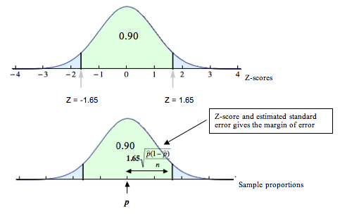
Technology is used to determine the z-scores that mark off the middle 90% of the sampling distribution. The z-scores are ±1.65. Using this value in place of 2 in the margin of error gives us a 90% confidence interval:
95% confidence interval: 0.533 ± 2(0.043) ≈ 0.533 ± 0.086 = (0.447, 0.619)
90% confidence interval: 0.533 ± 1.65(0.043) ≈ 0.533 ± 0.07 = (0.463, 0.603)
Note: Frequently, you will see the z-scores that mark off the middle 90% of the sample proportions represented more precisely as ±1.645.
What is the impact of decreasing the confidence level to 90%?
The 90% interval allows a smaller margin for error than the 95% interval. The 90% confidence interval is narrower than the 95% confidence interval. It may seem like an advantage, but there is a trade-off because we now have less confidence that the interval contains the population proportion. This is an important point. Lower confidence means smaller margin of error. We investigate this idea in more depth later.
Confidence Interval Formula
Since we are no longer restricting our confidence level to 95%, we can generalize the formula for a confidence interval:
[latex]\stackrel{ˆ}{p}\text{}±\text{}{Z}_{c}\sqrt{\frac{\stackrel{ˆ}{p}(1-\stackrel{ˆ}{p}}{n}}[/latex]
We use a little subscript c on the z-score, Zc , to emphasize that the z-score is connected to the confidence level. When giving the value of Zc, we always use the positive z-score.
Learn By Doing
Comment
Technology often uses 3 decimal places for Zc.
For our most common confidence levels, the values of Zc are:
- 90% confidence interval: Zc ≈ 1.645
- 95% confidence interval: Zc ≈ 1.960 (2 is a rough approximation; 1.960 is more accurate)
- 99% confidence interval: Zc ≈ 2.576
So when you calculate the confidence interval, rounding will slightly affect the values in your interval.
Candela Citations
- Concepts in Statistics. Provided by: Open Learning Initiative. Located at: http://oli.cmu.edu. License: CC BY: Attribution