Bounded Exponential Growth and Decay

Using Newton’s Law of Cooling

Exponential decay can also be applied to temperature. When a hot object is left in surrounding air that is at a lower temperature, the object’s temperature will decrease exponentially, leveling off as it approaches the surrounding air temperature. On a graph of the temperature function, the leveling off will correspond to a horizontal asymptote at the temperature of the surrounding air. Unless the room temperature is zero, this will correspond to a vertical shift of the generic exponential decay function. This translation leads to Newton’s Law of Cooling, the scientific formula for temperature as a function of time as an object’s temperature is equalized with the ambient temperature.

The formula is derived as follows:

[latex]\begin{array}{l}T\left(t\right)=A{b}^{ct}+{T}_{s}\hfill & \hfill \\ T\left(t\right)=A{e}^{\mathrm{ln}\left({b}^{ct}\right)}+{T}_{s}\hfill & \text{Properties of logarithms}.\hfill \\ T\left(t\right)=A{e}^{ct\mathrm{ln}b}+{T}_{s}\hfill & \text{Properties of logarithms}.\hfill \\ T\left(t\right)=A{e}^{kt}+{T}_{s}\hfill & \text{Rename the constant }c \mathrm{ln} b,\text{ calling it }k.\hfill \end{array}[/latex]

Logistic Models

Exponential growth cannot continue forever. Exponential models, while they may be useful in the short term, tend to fall apart the longer they continue. Consider an aspiring writer who writes a single line on day one and plans to double the number of lines she writes each day for a month. By the end of the month, she must write over 17 billion lines or one-half-billion pages. It is impractical, if not impossible, for anyone to write that much in such a short period of time. Eventually an exponential model must begin to approach some limiting value and then the growth is forced to slow. For this reason, it is often better to use a model with an upper bound instead of an exponential growth model although the exponential growth model is still useful over a short term before approaching the limiting value.

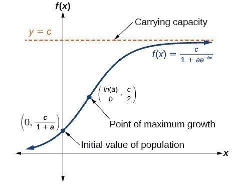
The logistic growth model is approximately exponential at first, but it has a reduced rate of growth as the output approaches the model’s upper bound called the carrying capacity. For constants a, b, and c, the logistic growth of a population over time x is represented by the model

[latex]f\left(x\right)=\frac{c}{1+a{e}^{-bx}}[/latex]

The graph below shows how the growth rate changes over time. The graph increases from left to right, but the growth rate only increases until it reaches its point of maximum growth rate at which the rate of increase decreases.

Example: Using the Logistic-Growth Model

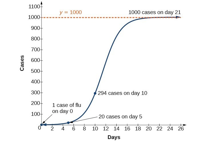
An influenza epidemic spreads through a population rapidly at a rate that depends on two factors. The more people who have the flu, the more rapidly it spreads, and also the more uninfected people there are, the more rapidly it spreads. These two factors make the logistic model good for studying the spread of communicable diseases. And, clearly, there is a maximum value for the number of people infected: the entire population.

For example, at time t = 0 there is one person in a community of 1,000 people who has the flu. So, in that community, at most 1,000 people can have the flu. Researchers find that for this particular strain of the flu, the logistic growth constant is b = 0.6030. Estimate the number of people in this community who will have had this flu after ten days. Predict how many people in this community will have had this flu after a long period of time has passed.

Show Solution

We substitute the given data into the logistic growth model

[latex]f\left(x\right)=\frac{c}{1+a{e}^{-bx}}[/latex]

Because at most 1,000 people, the entire population of the community, can get the flu, we know the limiting value is c = 1000. To find a, we use the formula that the number of cases at time t = 0 is [latex]\frac{c}{1+a}=1[/latex], from which it follows that a = 999. This model predicts that, after ten days, the number of people who have had the flu is [latex]f\left(x\right)=\frac{1000}{1+999{e}^{-0.6030x}}\approx 293.8[/latex]. Because the actual number must be a whole number (a person has either had the flu or not) we round to 294. In the long term, the number of people who will contract the flu is the limiting value, c = 1000.

Analysis of the Solution

Remember that because we are dealing with a virus, we cannot predict with certainty the number of people infected. The model only approximates the number of people infected and will not give us exact or actual values.

The graph below gives a good picture of how this model fits the data.

The graph of [latex]f\left(x\right)=\frac{1000}{1+999{e}^{-0.6030x}}[/latex].

Key Equations

Key Concepts

• We can use Newton’s Law of Cooling to find how long it will take for a cooling object to reach a desired temperature or to find what temperature an object will be after a given time.
• We can use logistic growth functions to model real-world situations where the rate of growth changes over time, such as population growth, spread of disease, and spread of rumors.

Glossary

carrying capacity

in a logistic model, the limiting value of the output

logistic growth model

a function of the form [latex]f\left(x\right)=\frac{c}{1+a{e}^{-bx}}[/latex] where [latex]\frac{c}{1+a}[/latex] is the initial value, c is the carrying capacity, or limiting value, and b is a constant determined by the rate of growth

Newton’s Law of Cooling

the scientific formula for temperature as a function of time as an object’s temperature is equalized with the ambient temperature