Learning Objectives
- Determine the pattern of exponential growth
- Define and graph exponential functions
- Describe the asymptote of an exponential function
- Find the domain and range of an exponential function
Exponential Growth
In Chapter 2, we looked at linear growth where there is a constant rate of change. Unlike linear growth that increases by adding a constant value to [latex]y[/latex] for every unit increase in [latex]x[/latex], exponential growth increases by multiplying by a constant that is neither equal to 0 nor 1. Table 1 shows exponential growth as each [latex]y[/latex]-value increases by a multiple of 2. Notice that the values in the [latex]x[/latex] column correspond to the exponents in the fourth column. This is because the values in the [latex]x[/latex] column record the number of times we have multiplied by 2.
| [latex]x[/latex] | [latex]y[/latex] | Number of times 2 gets multiplied | Exponential Notation |
|---|---|---|---|
| 1 | 2 | [latex]= 2[/latex] | [latex]=2^1[/latex] |
| 2 | 4 | [latex]= 2 \cdot 2[/latex] | [latex]=2^2[/latex] |
| 3 | 8 | [latex]= 2 \cdot 2 \cdot 2[/latex] | [latex]=2^3[/latex] |
| 4 | 16 | [latex]=2 \cdot 2 \cdot 2 \cdot 2[/latex] | [latex]=2^4[/latex] |
| 5 | 32 | [latex]=2 \cdot 2 \cdot 2 \cdot 2 \cdot 2[/latex] | [latex]=2^5[/latex] |
| Table 1. Exponential growth | |||
The pattern shown in the fourth column of table 1 indicates that exponential growth is repeated multiplication by a factor of 2 so the equation for the pattern is [latex]y= 2^x[/latex].
Zero and Negative Exponents
Table 1 shows the pattern of exponential growth of [latex]2^x[/latex] when [latex]x[/latex] is a natural number. But what is the value of [latex]2^x[/latex] when the exponent [latex]x[/latex] is zero or a negative number? If we consider the pattern in Table 1 in the reverse direction we can find the value of [latex]y=2^x[/latex] when [latex]x=0, -1, -2,...[/latex]. As the exponent decreases by 1, the value of [latex]y=2^x[/latex] is divided by 2.
For example, [latex]2^x=8[/latex] when the exponent [latex]x[/latex] is 3 (i.e., [latex]y=2^3=8[/latex]). As [latex]x[/latex] decreases by 1 to 2, the [latex]y[/latex] value is 4 (See Table 2). In other words, 8 is divided by 2 to get 4. Following this logic, the [latex]y[/latex] value will be 4 ÷ 2 = 2 when [latex]x[/latex] decreases by 1 again to 1. Following this pattern, the [latex]y[/latex] value will be 2 ÷ 2 = 1 when [latex]x[/latex] decreases by 1 again to zero. Therefore, [latex]2^0=1[/latex]. In fact, [latex]a^0=1[/latex] for all values of [latex]a[/latex], [latex]a\ne 0[/latex]. [latex]0^0[/latex] is undefined.
Exponent of Zero
[latex]a^0=1[/latex] for all values of [latex]a[/latex], [latex]a\ne 0[/latex]. [latex]0^0[/latex] is undefined.
Continuing this reverse pattern, the value of [latex]y[/latex] will be [latex]1\div 2=\dfrac{1}{2}[/latex] when [latex]x=-1[/latex]. Then, dividing by 2 again gives [latex]y=\dfrac{1}{2}÷2=\dfrac{1}{2}\cdot\dfrac{1}{2}=\dfrac{1}{4}[/latex] when [latex]x=-2[/latex]. Recall that dividing by 2 is equivalent to multiplying by [latex]\dfrac{1}{2}[/latex]. This pattern shows that the value of [latex]y[/latex] is a fraction where [latex]y=\dfrac{1}{2^{|x|}}[/latex] when the exponent [latex]x[/latex] is a negative number (See Table 2). For example, [latex]y=2^{-3}=\dfrac{1}{2^{|-3|}}=\dfrac{1}{2^3}[/latex]. In fact, the value of [latex]y=a^x[/latex] will alway be [latex]\dfrac{1}{a^{|x|}}[/latex] when the exponent [latex]x[/latex] is a negative number and the base [latex]a ≥ 0[/latex].
Negative Exponents
[latex]y=a^x=\dfrac{1}{a^{|x|}}[/latex] when the exponent [latex]x[/latex] is a negative number and [latex]a ≥ 0[/latex].
Table 3 shows how the values of [latex]y=2^x[/latex] for the exponents [latex]x=0, -1, -2, -3...[/latex] are obtained following the reverse pattern starting at [latex]x=0[/latex].
| [latex]x[/latex] | [latex]y[/latex] | Method for Obtaining [latex]y[/latex] | Equation |
|---|---|---|---|
| -3 | [latex]\dfrac{1}{8}[/latex] | [latex]=\dfrac{1}{2} \cdot \dfrac{1}{2} \cdot \dfrac{1}{2}[/latex] | [latex]2^{-3}[/latex] |
| -2 | [latex]\dfrac{1}{4}[/latex] | [latex]=\dfrac{1}{2} \cdot \dfrac{1}{2}[/latex] | [latex]2^{-2}[/latex] |
| -1 | [latex]\dfrac{1}{2}[/latex] | [latex]=\dfrac{1}{2}[/latex] | [latex]2^{-1}[/latex] |
| 0 | 1 | [latex]= 2 \cdot \dfrac{1}{2}[/latex] = 1 | [latex]2^0[/latex] |
| 1 | 2 | [latex]=2[/latex] | [latex]2^1[/latex] |
| 2 | 4 | [latex]= 2 \cdot 2[/latex] | [latex]2^2[/latex] |
| 3 | 8 | [latex]=2 \cdot 2 \cdot 2[/latex] | [latex]2^3[/latex] |
| 4 | 16 | [latex]=2 \cdot 2 \cdot 2 \cdot 2[/latex] | [latex]2^4[/latex] |
| 5 | 32 | [latex]=2 \cdot 2 \cdot 2 \cdot 2 \cdot 2[/latex] | [latex]2^5[/latex] |
| Table 2. Exponential growth with base 2 | |||
Zero and negative exponents will be discussed again in section 5.3.2 using the Product and Quotient Rule for Exponents.
Example 1
Complete the table for the equation [latex]y=10^x[/latex].
| [latex]x[/latex] | [latex]y[/latex] | Method for Obtaining [latex]y[/latex] | Equation |
|---|---|---|---|
| -3 | [latex]y=10^{-3}[/latex] | ||
| -2 | [latex]y=10^{-2}[/latex] | ||
| -1 | [latex]y=10^{-1}[/latex] | ||
| 0 | [latex]y=10^0[/latex] | ||
| 1 | 10 | [latex]= 10[/latex] | [latex]y=10^1[/latex] |
Solution
Since the base of the function is 10, we divide the [latex]y[/latex]-value by 10 as [latex]x[/latex] decreases by 1.
| [latex]x[/latex] | [latex]y[/latex] | Method for Obtaining [latex]y[/latex] | Equation |
|---|---|---|---|
| -3 | [latex]\dfrac{1}{1000}[/latex] | [latex]\dfrac{1}{100}\div10=\dfrac{1}{1000}[/latex] | [latex]y=10^{-3}[/latex] |
| -2 | [latex]\dfrac{1}{100}[/latex] | [latex]\dfrac{1}{10}\div10=\dfrac{1}{100}[/latex] | [latex]y=10^{-2}[/latex] |
| -1 | [latex]\dfrac{1}{10}[/latex] | [latex]1\div10=\dfrac{1}{10}[/latex] | [latex]y=10^{-1}[/latex] |
| 0 | 1 | [latex]10\div10=1[/latex] | [latex]y=10^0[/latex] |
| 1 | 10 | [latex]= 10[/latex] | [latex]y=10^1[/latex] |
Try It 1
Complete the table for the equation [latex]y=3^x[/latex].
| [latex]x[/latex] | [latex]y[/latex] | Method for Obtaining [latex]y[/latex] | Equation |
|---|---|---|---|
| -3 | [latex]y=3^{-3}[/latex] | ||
| -2 | [latex]y=3^{-2}[/latex] | ||
| -1 | [latex]y=3^{-1}[/latex] | ||
| 0 | [latex]y=3^0[/latex] | ||
| 1 | 3 | [latex]3[/latex] | [latex]y=3^1[/latex] |
Solution
Since the base of the function is 3, we divide the [latex]y[/latex]-value by 3 as [latex]x[/latex] decreases by 1.
| [latex]x[/latex] | [latex]y[/latex] | Method for Obtaining [latex]y[/latex] | Equation |
|---|---|---|---|
| -3 | [latex]\dfrac{1}{27}[/latex] | [latex]\dfrac{1}{9}\div3=\dfrac{1}{27}[/latex] | [latex]y=3^{-3}[/latex] |
| -2 | [latex]\dfrac{1}{9}[/latex] | [latex]\dfrac{1}{3}\div3=\dfrac{1}{9}[/latex] | [latex]y=3^{-2}[/latex] |
| -1 | [latex]\dfrac{1}{3}[/latex] | [latex]1\div3=\dfrac{1}{3}[/latex] | [latex]y=3^{-1}[/latex] |
| 0 | 1 | [latex]3\div3=1[/latex] | [latex]y=3^0[/latex] |
| 1 | 3 | [latex]=3[/latex] | [latex]y=3^1[/latex] |
Example 2
Evaluate [latex]y=4^x[/latex] when,
- a) [latex]x=1[/latex]
- b) [latex]x=3[/latex]
- c) [latex]x=0[/latex]
- d) [latex]x=-2[/latex]
- e) [latex]x=-3[/latex]
Solution
- a) [latex]4^1=4[/latex]
- b) [latex]4^3=4\cdot4\cdot4=64[/latex]
- c) [latex]4^0=1[/latex]
- d) [latex]4^{-2}=\dfrac{1}{4^2}=\dfrac{1}{16}[/latex]
- e) [latex]4^{-3}=\dfrac{1}{4^3}=\dfrac{1}{64}[/latex]
Try It 2
Evaluate [latex]y=7^x[/latex] when,
- a) [latex]x=1[/latex]
- b) [latex]x=2[/latex]
- c) [latex]x=0[/latex]
- d) [latex]x=-2[/latex]
- e) [latex]x=-3[/latex]
The Difference between Exponential Growth and Power Growth
In exponential growth, the variable is the exponent (e.g., [latex]2^x[/latex]). In power growth, the variable is the base (e.g., [latex]x^2[/latex]). Exponential growth grows faster than power growth. For example, table 3 shows that the exponential growth [latex]2^x[/latex] grows much faster than the power growth [latex]x^2[/latex] while table 4 shows that the exponential growth [latex]3^x[/latex] grows much faster than the power growth [latex]x^3[/latex].
| [latex]x[/latex] | [latex]x^2[/latex] | [latex]2^x[/latex] | ____ | [latex]x[/latex] | [latex]x^3[/latex] | [latex]3^x[/latex] |
|---|---|---|---|---|---|---|
| 0 | 0 | 1 | 0 | 0 | 1 | |
| 1 | 1 | 2 | 1 | 1 | 3 | |
| 2 | 4 | 4 | 2 | 8 | 9 | |
| 3 | 9 | 8 | 3 | 27 | 27 | |
| 4 | 16 | 16 | 4 | 64 | 81 | |
| 5 | 25 | 32 | 5 | 125 | 243 | |
| 6 | 36 | 64 | 6 | 216 | 729 | |
| 7 | 49 | 128 | 7 | 343 | 2187 | |
| 8 | 64 | 256 | 8 | 512 | 6561 | |
| Table 3. Exponential versus power growth | Table 4. Exponential versus power growth | |||||
Initial Value
The initial value of exponential growth occurs at [latex]x=0[/latex]. So far we have considered only initial values of 1. Tables 1 and 2 show a pattern where [latex]y=1\cdot 2^x[/latex]. However, the initial value can be any real number.
For example, let’s consider an initial value of 8 and an exponential growth rate of 2. We can create a table that illustrates this scenario starting with [latex]y=8[/latex] when [latex]x=0[/latex], then multiplying each [latex]y[/latex]-value by 2:
| [latex]x[/latex] | [latex]y[/latex] | Equation |
|---|---|---|
| -2 | [latex]4\div 2=2[/latex] | [latex]8\cdot2^{-2}[/latex] |
| -1 | [latex]8\div 2=4[/latex] | [latex]8\cdot2^{-1}[/latex] |
| 0 | [latex]8[/latex] | [latex]y=8\cdot2^0[/latex] |
| 1 | [latex]8\cdot 2=16[/latex] | [latex]8\cdot2^1[/latex] |
| 2 | [latex]16\cdot 2=32[/latex] | [latex]8\cdot2^2[/latex] |
| 3 | [latex]32\cdot 2=64[/latex] | [latex]8\cdot2^3[/latex] |
The equation that models an exponential growth rate of 2 with an initial value of 8 is [latex]y=8\cdot2^x[/latex].
Exponential Growth
The equation that models an exponential growth rate of [latex]r[/latex] with an initial value of [latex]a[/latex] is [latex]y=a\cdot r^x[/latex].
Example 3
Complete the table for an exponential growth of 4 and an initial value of 3. Then write an equation for the exponential growth pattern.
| [latex]x[/latex] | [latex]y[/latex] |
|---|---|
| [latex]–2[/latex] | |
| [latex]–1[/latex] | |
| [latex]0[/latex] | |
| [latex]1[/latex] | |
| [latex]2[/latex] | |
| [latex]3[/latex] |
Solution
The initial value of 3 occurs when [latex]x=0[/latex] so we can add that to the table. Then we can multiply by 4 each time to determine the [latex]y[/latex]-values for [latex]x=1,\;2[/latex]. To find the [latex]y[/latex]-values for [latex]x=-1,\;-2[/latex], we work backwards by dividing the initial value by 4.
| [latex]x[/latex] | [latex]y[/latex] |
|---|---|
| [latex]–2[/latex] | [latex]3÷4÷4=\dfrac{3}{16}[/latex] |
| [latex]–1[/latex] | [latex]3÷4=\dfrac{3}{4}[/latex] |
| [latex]0[/latex] | [latex]3[/latex] |
| [latex]1[/latex] | [latex]3\cdot 4=12[/latex] |
| [latex]2[/latex] | [latex]3\cdot 4\cdot 4=48[/latex] |
| [latex]3[/latex] | [latex]3\cdot 4\cdot 4\cdot 4=192[/latex] |
The pattern is [latex]y=3\cdot 4^x[/latex]
Try It 3
Complete the table for an exponential growth of 3 and an initial value of 5. Then write an equation for the exponential growth pattern.
Try It 4
Write an equation for the following exponential growth patterns:
- growth = 6; initial value = 4
- growth = 2; initial value = 9
- growth = [latex]\dfrac{2}{3}[/latex]; initial value = 5
- growth = 0.77; initial value = –5.4
Exponential Functions and Their Graphs
Exponential growth has an initial value and an exponential rate of change. The initial value occurs at [latex]x=0[/latex]. In table 1, the initial value is 1 (when [latex]x=0[/latex]), and the exponential rate of change is 2. This creates a pattern where [latex]y=1\cdot 2^x[/latex]. Consequently, the exponential growth in table 1 may be modeled or represented by the function [latex]f(x) = 2^x[/latex].
If we graph the values [latex](x, y)[/latex] from table 1, we can then connect the points to draw the graph the exponential function [latex]f(x)=2^x[/latex] (figure 1).
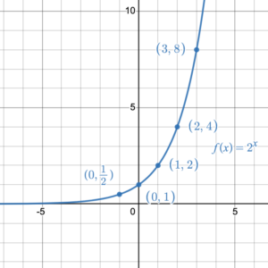
Figure 1. The graph of the function [latex]f(x)=2^x[/latex].
Example 4
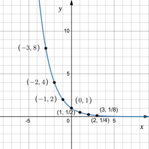
Create a table of values then graph the function [latex]f(x)=\left(\dfrac{1}{2}\right)^x[/latex].
Solution
We can choose any [latex]x[/latex]-values to create a table for [latex]y=f(x)[/latex]:
| [latex]x[/latex] | [latex]y[/latex] |
|---|---|
| [latex]0[/latex] | [latex]\left(\dfrac{1}{2}\right)^0=1[/latex] |
| [latex]1[/latex] | [latex]\left(\dfrac{1}{2}\right)^1=\dfrac{1}{2}[/latex] |
| [latex]2[/latex] | [latex]\left(\dfrac{1}{2}\right)^2=\dfrac{1}{4}[/latex] |
| [latex]-1[/latex] | [latex]\left(\dfrac{1}{2}\right)^{-1}=2^1=2[/latex] |
| [latex]-2[/latex] | [latex]\left(\dfrac{1}{2}\right)^{-2}=2^2=4[/latex] |
| [latex]-3[/latex] | [latex]\left(\dfrac{1}{2}\right)^{-3}=2^3=8[/latex] |
We plot the [latex](x,y)[/latex] points from the table:

Then join the points with a smooth curve:
Try It 5
Create a table of values then graph the function [latex]f(x)=4^x[/latex].

The Definition of an Exponential Function
An exponential function has the form [latex]f(x) = r^x[/latex], where [latex]r[/latex] is a real number with [latex]r >0[/latex] and [latex]r \neq 1[/latex].
Figure 2 illustrates how the graph changes as the value of [latex]r[/latex] changes. Move the red circle up or down to change the value of [latex]r[/latex] and watch what happens to the function.
Figure 2. Interactive graph [latex]f(x)=r^x[/latex]
Manipulate the graph of [latex]f(x)=r^x[/latex] in figure 2 to answer the following questions:
1. What happens to the point (0, 1) as [latex]r[/latex]changes?
The point (0, 1) never changes. The point (0, 1) is always on the graph of [latex]f(x)=r^x[/latex].
2. What happens to the point on the graph at [latex]x=1[/latex] as [latex]r[/latex]changes?
At [latex]x=1[/latex], the point on the graph will always be [latex](1, r)[/latex], because [latex]f(1)=r^1=r[/latex].
3. What happens to the graph when [latex]r=1[/latex]?
If [latex]r=1[/latex] we get a flat line; a linear equation [latex]y=1[/latex]. This is why [latex]r[/latex] is never allowed to equal 1.
4. What happens to the graph when [latex]r=0[/latex]?
If [latex]r=0[/latex] we get a flat line starting at [latex]x>0[/latex]. [latex]f(0)=0^0[/latex] which is undefined. For any [latex]x<0[/latex], [latex]0^{\text{negative number}}=\dfrac{1}{0^{\text{positive number}}}=\dfrac{1}{0}[/latex], which is undefined. This is why [latex]r[/latex] is never allowed to equal 0.
5. What happens to the graph when [latex]r<0[/latex]?
When [latex]r<0[/latex], the graph disappears!! This is why [latex]r[/latex] is a positive real number ≠ 0, 1.
6. What happens to the graph when [latex]r>1[/latex]?
The graph comes up from [latex]y=0[/latex], passes through (0, 1) and (1, r), then quickly moves towards [latex]+\infty[/latex].
7. What happens to the graph when [latex]0
The Asymptote and Intercepts
A significant feature on the graph of any exponential function [latex]f(x) = r^x[/latex] ([latex]r>0,\;r\neq1[/latex]) is that the graph never crosses the [latex]x[/latex]-axis. It continually approaches the [latex]x[/latex], getting closer and closer, but the graph never meets the [latex]x[/latex]-axis. Figure 2 illustrates that when [latex]0
| Graphs with horizontal asymptotes | |
|---|---|
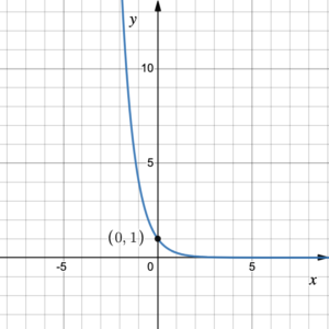 |
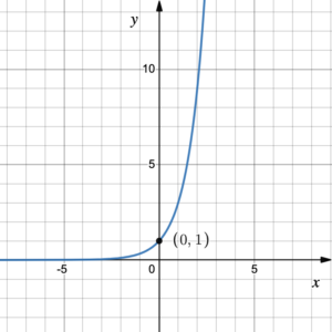 |
Figure 3. [latex]f(x)=r^x[/latex] with [latex]0| Figure 4. [latex]f(x)=r^x[/latex] with [latex]r>1[/latex] |
|
Why does the graph never meet the [latex]x[/latex]-axis? Consider the following examples using the function [latex]f(x)=2^x[/latex] that was graphed in figure 1:
[latex]f(-10)=2^{-10}=\dfrac{1}{2^{10}}[/latex]
[latex]f(-100)=2^{-100}=\dfrac{1}{2^{100}}[/latex]
[latex]f(-100000)=2^{-100000}=\dfrac{1}{2^{100000}}[/latex]
As the the value of [latex]x[/latex] gets closer to negative infinity, the value of the function [latex]y[/latex] is a fraction with a numerator of 1 and a denominator that is a very large positive number. The value of [latex]x[/latex] gets more and more negative as it gets closer to negative infinity, so the value of the function will get smaller and smaller. It will get close to zero but will never be zero because [latex]\dfrac{1}{\text{very large positive number}}[/latex] is always positive and therefore greater than zero.
Figure 2 shows that for all values of [latex]r>0[/latex] and [latex]r\neq1[/latex], the graph gets close to but never crosses the [latex]x[/latex]-axis, it is a horizontal asymptote of the function [latex]f(x)=r^x[/latex]. Also, since the graph never meets the [latex]x[/latex]-axis, there is no [latex]x[/latex]-intercept for the function. The [latex]y[/latex]-intercept of the function [latex]f(x)=r^x[/latex] is always (0, 1).
We use a dotted line to show that a graph has a horizontal asymptote (figure 5).
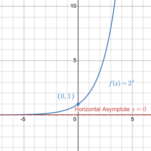
Figure 5. Exponential function with horizontal asymptote.
Domain and Range
Figure 5 shows the graph of [latex]f(x)=2^x[/latex]. The domain of the function is the set of all possible [latex]x[/latex]-values, so domain = [latex]\{x\;|\;x\in \mathbb{R}\}[/latex]. Any [latex]x[/latex]-value from [latex]-\infty[/latex] to [latex]+\infty[/latex] has a corresponding function value. It’s range, the set of all function values, lies above the line [latex]y=0[/latex]. Consequently, the range =[latex]\{f(x)\;|\;f(x)\in\mathbb{R}^+\}[/latex], where [latex]\mathbb{R}^+[/latex] is the set of all positive real numbers.
DOMAIN and RANGE
The domain of any exponential function [latex]f(x)=r^x[/latex] is all real numbers, or [latex]\{x | x \in \mathbb{R}\}[/latex], or [latex](-\infty, \infty)[/latex]. The range of any exponential function[latex]f(x)=r^x[/latex] is all real numbers that are above the horizontal asymptote. Range = [latex]\{f(x)\;|\;f(x)\in\mathbb{R}^+\}[/latex], or [latex](0, \infty)[/latex].
The exponential function [latex]f(x)=r^x[/latex] is the parent function of all exponential functions. In the next section, we will see what happens to the graph of the function when we transform the parent function.
Candela Citations
- Exponential functions and Their Graphs. Authored by: Hazel McKenna and Leo Chang. Provided by: Utah Valley University. License: CC BY: Attribution
- All graphs created using desmos graphing calculator. Authored by: Hazel McKenna. Provided by: Utah Valley University. License: CC BY: Attribution
- All examples and Try its: hjm585; hjm469; hjm118. Authored by: Hazel McKenna. Provided by: Utah Valley University. License: CC BY: Attribution