Learning Objectives
For the rational parent function [latex]f(x)=\dfrac{1}{x}[/latex],
- Perform vertical and horizontal shifts
- Perform vertical stretches and compressions
- Perform reflections across the [latex]x[/latex]-axis
- Perform reflections across the [latex]y[/latex]-axis
- Determine the transformations performed on the parent function [latex]f(x)=\dfrac{1}{x}[/latex] to get the rational function [latex]f(x)=a\left(\dfrac{1}{x-h}\right)+k[/latex]
Vertical Shifts
If we shift the graph of the rational function [latex]f(x)=\dfrac{1}{x}[/latex] up 5 units, all of the points on the graph increase their [latex]y[/latex]-coordinates by 5, but their [latex]x[/latex]-coordinates remain the same. Therefore, the equation of the function [latex]f(x)=\dfrac{1}{x}[/latex] after it has been shifted up 5 units transforms to [latex]f(x)=\dfrac{1}{x}+5[/latex]. Table 1 shows the changes to specific values of this function, which are replicated on the graph in figure 1.
| [latex]x[/latex] | [latex]\dfrac{1}{x}[/latex] | [latex]\dfrac{1}{x}+5[/latex] |
Figure 1. Shifting the graph of the function [latex]f(x)=\frac{1}{x}[/latex] up 5 units. |
|---|---|---|---|
| [latex]–2[/latex] | [latex]-\dfrac{1}{2}[/latex] | [latex]\dfrac{9}{2}[/latex] | |
| [latex]–1[/latex] | [latex]–1[/latex] | [latex]4[/latex] | |
| [latex]-\dfrac{1}{2}[/latex] | [latex]–2[/latex] | [latex]3[/latex] | |
| [latex]\dfrac{1}{2}[/latex] | [latex]2[/latex] | [latex]7[/latex] | |
| [latex]1[/latex] | [latex]1[/latex] | [latex]6[/latex] | |
| [latex]2[/latex] | [latex]\dfrac{1}{2}[/latex] | [latex]\dfrac{11}{2}[/latex] | |
| [latex]3[/latex] | [latex]\dfrac{1}{3}[/latex] | [latex]\dfrac{16}{3}[/latex] | |
| Table 1. [latex]f(x)=\frac{1}{x}[/latex] is transformed to[latex]f(x)=\frac{1}{x}+5[/latex]. | |||

If we shift the graph of the function [latex]f(x)=\frac{1}{x}[/latex] down 8 units, all of the points on the graph decrease their [latex]y[/latex]-coordinates by 8, but their [latex]x[/latex]-coordinates remain the same. Therefore, the equation of the function [latex]f(x)=\frac{1}{x}[/latex] after it has been shifted down 8 units transforms to [latex]f(x)=\frac{1}{x}-8[/latex]. Table 2 shows the changes to specific values of this function, which are replicated on the graph in figure 2.
| [latex]f(x)[/latex] | [latex]\dfrac{1}{x}[/latex] | [latex]f(x)=\dfrac{1}{x}-8[/latex] |
Figure 2. Shifting the graph of the function [latex]f(x)=\frac{1}{x}[/latex] down 8 units. |
|---|---|---|---|
| [latex]–2[/latex] | [latex]-\dfrac{1}{2}[/latex] | [latex]-\dfrac{17}{2}[/latex] | |
| [latex]–1[/latex] | [latex]–1[/latex] | [latex]–9[/latex] | |
| [latex]-\dfrac{1}{2}[/latex] | [latex]–2[/latex] | [latex]–10[/latex] | |
| [latex]\dfrac{1}{2}[/latex] | [latex]2[/latex] | [latex]–6[/latex] | |
| [latex]1[/latex] | [latex]1[/latex] | [latex]–7[/latex] | |
| [latex]2[/latex] | [latex]\frac{1}{2}[/latex] | [latex]-\frac{15}{2}[/latex] | |
| [latex]3[/latex] | [latex]\frac{1}{3}[/latex] | [latex]-\frac{23}{3}[/latex] | |
| Table 2. [latex]f(x)=\frac{1}{x}[/latex] is transformed to [latex]f(x)=\frac{1}{x}-8[/latex]. | |||

Vertical shifts
We can represent a vertical shift of the graph of the function [latex]f(x)=\dfrac{1}{x}[/latex] by adding a constant, [latex]k[/latex], to the function:
[latex]f(x)=\dfrac{1}{x}+k[/latex]
If [latex]k>0[/latex], the graph shifts upwards and if [latex]k<0[/latex] the graph shifts downwards.
Manipulate the graph in figure 3 to shift the graph vertically. Pay attention to what happens with the function as [latex]k[/latex] changes value. Also, watch what happens with the asymptotes.
Figure 3. Vertical Transformations
Example 1
- Use figure 3 to graph the function [latex]f(x)=\frac{1}{x}-6[/latex]. What is the horizontal asymptote of the function? What is the relationship between the value of [latex]k[/latex] and the horizontal asymptote? What is the vertical asymptote of the function?
- Without graphing the function, what is the horizontal asymptote of the function [latex]g(x)=\frac{1}{x}+5[/latex]? What is the vertical asymptote?
Solution
1.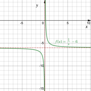
The horizontal asymptote is the line [latex]y=-6[/latex]. The value of [latex]k[/latex] is [latex]-6[/latex] so the horizontal asymptote mimics the value of [latex]k[/latex].
The vertical asymptote is the line [latex]x=0[/latex].
2. Since [latex]k=5[/latex] the graph of [latex]f(x)=\frac{1}{x}[/latex] gets shifted up by 5 units. This means that the horizontal asymptote is shifted up 5 units to [latex]y=5[/latex]. The vertical asymptote does not move so is still [latex]x=0[/latex].
Try It 1
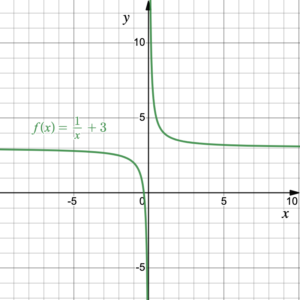
- Use figure 3 to graph the function [latex]f(x)=\frac{1}{x}+3[/latex]. What is the horizontal asymptote of the function? What is the relationship between the value of [latex]k[/latex] and the horizontal asymptote? What is the vertical asymptote of the function?
- Without graphing the function, what is the horizontal asymptote of the function [latex]g(x)=\frac{1}{x}-7[/latex]? What is the vertical asymptote?
Example 2
The graph of the rational function [latex]y=f(x)[/latex] has a horizontal asymptote at [latex]y=9[/latex] and a vertical asymptote at [latex]x=0[/latex]. Determine a rational functional [latex]f(x)[/latex] whose graph meets these criteria.
Solution
Since the vertical asymptote is at [latex]x=0[/latex] there is no horizontal shift from the parent function [latex]f(x)=\dfrac{1}{x}[/latex]. Since the horizontal asymptote is at [latex]y=9[/latex], there has been a vertical shift of 9 units up from the parent function [latex]f(x)=\dfrac{1}{x}[/latex]. This means that [latex]k=9[/latex], and the function is [latex]f(x)=\dfrac{1}{x}+9[/latex].
Try It 2
The graph of the rational function [latex]y=f(x)[/latex] has a horizontal asymptote at [latex]y=-12[/latex] and a vertical asymptote at [latex]x=0[/latex]. Determine a rational functional [latex]f(x)[/latex] whose graph meets these criteria.
Horizontal Shifts
If we shift the graph of the function [latex]f(x)=\dfrac{1}{x}[/latex] right 7 units, all of the points on the graph increase their [latex]x[/latex]-coordinates by 7, but their [latex]y[/latex]-coordinates remain the same. The point (1, 1) in the original graph is moved to (8, 1). Any point [latex](x, y)[/latex] on the original graph is moved to [latex](x+7, y)[/latex](figure 4).
But what happens to the original function [latex]f(x)=\dfrac{1}{x}[/latex]? An automatic assumption may be that since [latex]x[/latex] moves to [latex]x+7[/latex] that the function will become [latex]f(x)=\dfrac{1}{x+7}[/latex]. But that is NOT the case. Remember that the [latex]x[/latex]-intercept is moved to (8, 1) and if we substitute [latex]x=8[/latex] into the function [latex]f(x)=\dfrac{1}{x+7}[/latex] we get [latex]f(x)=\dfrac{1}{15} \neq 1[/latex]!! The way to get a function value of 1 is for the transformed function to be [latex]f(x)=\dfrac{1}{x-7}[/latex]. Then[latex]f(8)=\dfrac{1}{8-7}=1[/latex]. So the function [latex]f(x)=\dfrac{1}{x}[/latex] transforms to [latex]f(x)=\dfrac{1}{x-7}[/latex] after being shifted 7 units to the right. The reason is that when we move the function 7 units to the right, the [latex]x[/latex]-value increases by 7 and to keep the corresponding [latex]y[/latex]-coordinate the same in the transformed function, the [latex]x[/latex]-coordinate of the transformed function needs to subtract 7 to get back to the original [latex]x[/latex] that is associated with the original [latex]y[/latex]-value. Table 3 shows the changes to specific values of this function, and the graph is shown in figure 4.
| [latex]x[/latex] | [latex]x-7[/latex] | [latex]f(x)=\dfrac{1}{x-7}[/latex] | 
Figure 4. Shifting the graph of the function [latex]f(x)=\frac{1}{x}[/latex] right 7 units. |
|---|---|---|---|
| [latex]5[/latex] | [latex]-2[/latex] | [latex]-\frac{1}{2}[/latex] | |
| [latex]6[/latex] | [latex]-1[/latex] | [latex]-1[/latex] | |
| [latex]\frac{13}{2}[/latex] | [latex]-\frac{1}{2}[/latex] | [latex]-2[/latex] | |
| [latex]\frac{15}{2}[/latex] | [latex]\frac{1}{2}[/latex] | [latex]2[/latex] | |
| [latex]8[/latex] | [latex]1[/latex] | [latex]1[/latex] | |
| [latex]9[/latex] | [latex]2[/latex] | [latex]\frac{1}{2}[/latex] | |
| [latex]10[/latex] | [latex]3[/latex] | [latex]\frac{1}{3}[/latex] | |
| Table 3. Shifting the graph right by 7 units transforms [latex]f(x)=\frac{1}{x}[/latex] into [latex]f(x)=\frac{1}{x-7}[/latex] . | |||
On the other hand, if we shift the graph of the function [latex]f(x)=\dfrac{1}{x}[/latex] left by 11 units, all of the points on the graph decrease their [latex]x[/latex]-coordinates by 11, but their [latex]y[/latex]-coordinates remain the same. So any point [latex](x, y)[/latex] on the original graph moves to [latex](x-11, y)[/latex]. Consequently, to keep the same [latex]y[/latex]-values we need to increase the [latex]x[/latex]-value by 11 in the transformed function. The equation of the function after being shifted left 11 units is [latex]f(x)=\dfrac{1}{x+11}[/latex]. Table 4 shows the changes to specific values of this function, and the graph is shown in figure 5.
| [latex]x[/latex] | [latex]x+11[/latex] | [latex]f(x)=\dfrac{1}{x+11}[/latex] |
Figure 5. Shifting the graph of the function [latex]f(x)=\dfrac{1}{x}[/latex] left 11 units. |
|---|---|---|---|
| [latex]–13[/latex] | [latex]-2[/latex] | [latex]-\frac{1}{2}[/latex] | |
| [latex]-12[/latex] | [latex]-1[/latex] | [latex]-1[/latex] | |
| [latex]-\frac{23}{2}[/latex] | [latex]-\frac{1}{2}[/latex] | [latex]-2[/latex] | |
| [latex]-\frac{21}{2}[/latex] | [latex]\frac{1}{2}[/latex] | [latex]2[/latex] | |
| [latex]-10[/latex] | [latex]1[/latex] | [latex]1[/latex] | |
| [latex]-9[/latex] | [latex]2[/latex] | [latex]\frac{1}{2}[/latex] | |
| [latex]-8[/latex] | [latex]3[/latex] | [latex]\frac{1}{3}[/latex] | |
| Table 4. Shifting the graph left by 11 units transforms [latex]f(x)=\dfrac{1}{x}[/latex] into [latex]f(x)=\dfrac{1}{x+11}[/latex]. | |||

horizontal shifts
We can represent a horizontal shift of the graph of the function [latex]f(x)=\dfrac{1}{x}[/latex] by subtracting a constant, [latex]h[/latex], from the variable [latex]x[/latex].
[latex]f(x)=\dfrac{1}{x-h}[/latex]
If [latex]h>0[/latex] the graph shifts toward the right and if [latex]h<0[/latex] the graph shifts to the left.
Manipulate the graph in figure 6 to shift the graph horizontally. Pay attention to what happens with the function as [latex]h[/latex] changes value. Also, watch what happens with the asymptotes.
Figure 6. Horizontal shifts
Example 3
- Use figure 6 to graph the function [latex]f(x)=\frac{1}{x+6}[/latex]. What is the vertical asymptote of the function? What is the relationship between the value of [latex]h[/latex] and the vertical asymptote? What is the horizontal asymptote of the function?
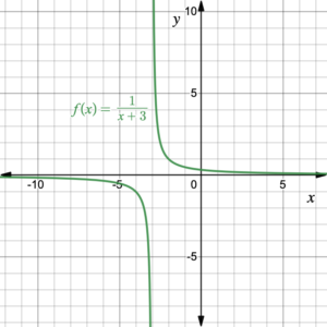
- Without graphing the function, what is the vertical asymptote of the function [latex]g(x)=\frac{1}{x+3}[/latex]? What is the horizontal asymptote?
Solution
1. 
The vertical asymptote is the line [latex]x=-6[/latex]. The value of [latex]h[/latex] is [latex]-6[/latex] so the vertical asymptote mimics the value of [latex]h[/latex].
The horizontal asymptote is the line [latex]y=0[/latex].
2. Since [latex]h=-3[/latex] the graph of [latex]f(x)=\frac{1}{x}[/latex] gets shifted left by 3 units. This means that the vertical asymptote is shifted left 3 units to [latex]x=-3[/latex]. The horizontal asymptote does not move so is still [latex]y=0[/latex].
Try It 3
- Use figure 6 to graph the function [latex]f(x)=\frac{1}{x+3}[/latex]. What is the vertical asymptote of the function? What is the relationship between the value of [latex]h[/latex] and the vertical asymptote? What is the horizontal asymptote of the function?
- Without graphing the function, what is the vertical asymptote of the function [latex]g(x)=\frac{1}{x-7}[/latex]? What is the horizontal asymptote?
Example 4
The graph of the rational function [latex]y=f(x)[/latex] has a horizontal asymptote at [latex]y=0[/latex] and a vertical asymptote at [latex]x=5[/latex]. Determine a rational functional [latex]f(x)[/latex] whose graph meets these criteria.
Solution
Since the horizontal asymptote is at [latex]y=0[/latex] there is no vertical shift from the parent function [latex]f(x)=\dfrac{1}{x}[/latex]. Since the vertical asymptote is at [latex]x=5[/latex], there has been a horizontal shift of 5 units right from the parent function [latex]f(x)=\dfrac{1}{x}[/latex]. This means that [latex]h=5[/latex], and the function is [latex]f(x)=\dfrac{1}{x-5}[/latex].
Try It 4
The graph of the rational function [latex]y=f(x)[/latex] has a horizontal asymptote at [latex]y=0[/latex] and a vertical asymptote at [latex]x=-9[/latex]. Determine a rational functional [latex]f(x)[/latex] whose graph meets these criteria.
Combining Vertical and Horizontal Shifts
vertical and horizontal shifts
We can represent both a vertical and a horizontal shift of the graph of the function [latex]f(x)=\dfrac{1}{x}[/latex] by the transformed function
[latex]f(x)=\dfrac{1}{x-h}+k[/latex]
If [latex]h>0[/latex] the graph shifts toward the right and if [latex]h<0[/latex] the graph shifts to the left. If [latex]k>0[/latex] the graph shifts upwards and if [latex]k<0[/latex] the graph shifts downwards.
When the parent function [latex]f(x)=\dfrac{1}{x}[/latex] is shifted both vertically and horizontally, there will be non-zero values for both [latex]h[/latex] and [latex]k[/latex]. The graph in figure 7 can be manipulated both vertically and horizontally. Pay attention to what happens to the function as the values for [latex]h[/latex] and [latex]k[/latex] change. Also notice what happens to the asymptotes.
Figure 7. Vertical and horizontal shifts
Example 5
The graph of the parent function [latex]f(x)=\dfrac{1}{x}[/latex] is shifted up by 4 units and left by 7 units.
- Determine the equation of the transformed function.
- Determine the vertical asymptote.
- Determine the horizontal asymptote.
- The point [latex](2, \frac{1}{2})[/latex] lies on the parent function. Where does it end up after the transformation?
Solution
- Shifted up by 4 units means [latex]k=4[/latex] and shifted left by 7 units means [latex]h=-7[/latex]. Therefore the function is [latex]f(x)=\dfrac{1}{x-h}+k=\dfrac{1}{x+7}+4[/latex].
- Since the graph is shifted left 7 units, the vertical asymptote is also shifted left 7 units: [latex]x=-7[/latex].
- Since the graph is shifted up 4 units, the horizontal asymptote is also shifted up 4 units: [latex]y=4[/latex].
- Since the graph is shifted left 7 units, the [latex]x[/latex]-coordinate is shifted left 7 units to 2 – 7 = –5. Since the graph is shifted up 4 units, the [latex]y[/latex]-coordinate is shifted up 4 units to [latex]\frac{1}{2}+4=\frac{9}{2}[/latex]. Consequently,[latex](2, \frac{1}{2})[/latex] moves to [latex](-5, \frac{9}{2})[/latex].
Try It 5
The graph of the parent function [latex]f(x)=\dfrac{1}{x}[/latex] is shifted down by 3 units and right by 2 units.
- Determine the equation of the transformed function.
- Determine the vertical asymptote.
- Determine the horizontal asymptote.The point [latex](2, \frac{1}{2})[/latex] lies on the parent function. Where does it end up after the transformation?
Stretching and Compressing
If we vertically stretch the graph of the function [latex]f(x)=\dfrac{1}{x}[/latex] by a factor of 7, all of the[latex]y[/latex]-coordinates of the points on the graph are multiplied by 7, but their [latex]x[/latex]-coordinates remain the same. The equation of the function after the graph is stretched is [latex]f(x)=7\times\dfrac{1}{x}=\dfrac{7}{x}[/latex]. The reason for multiplying [latex]f(x)=\dfrac{1}{x}[/latex] by 7 is that each [latex]y[/latex]-coordinate is made 7 times larger, and since [latex]y=\dfrac{1}{x}[/latex], [latex]\dfrac{1}{x}[/latex] is also made 7 times larger. Table 5 shows this change and the graph is shown in figure 8.
| [latex]x[/latex] | [latex]\dfrac{1}{x}[/latex] | [latex]f(x)=\dfrac{7}{x}[/latex] |
Figure 8. Stretching the graph vertically. |
|---|---|---|---|
| [latex]-2[/latex] | [latex]-\frac{1}{2}[/latex] | [latex]-\frac{7}{2}[/latex] | |
| [latex]-1[/latex] | [latex]-1[/latex] | [latex]-7[/latex] | |
| [latex]-\frac{1}{2}[/latex] | [latex]-2[/latex] | [latex]-14[/latex] | |
| [latex]\frac{1}{2}[/latex] | [latex]2[/latex] | [latex]14[/latex] | |
| [latex]1[/latex] | [latex]1[/latex] | [latex]7[/latex] | |
| [latex]2[/latex] | [latex]\dfrac{1}{2}[/latex] | [latex]\frac{7}{2}[/latex] | |
| [latex]3[/latex] | [latex]\dfrac{1}{3}[/latex] | [latex]\frac{7}{3}[/latex] | |
| Table 5. Stretching the graph vertically 7 times transforms [latex]\dfrac{1}{x}[/latex] into [latex]\dfrac{7}{x}[/latex]. | |||

On the other hand, if we vertically compress the graph of the function [latex]\dfrac{1}{x}[/latex] into [latex]\dfrac{1}{5}[/latex] of its original height, all of the [latex]y[/latex]-coordinates of the points on the graph are divided by 5, but their [latex]x[/latex]-coordinates remain the same. This means the [latex]y[/latex]-coordinates are multiplied by [latex]\dfrac{1}{5}[/latex]. The equation of the function after being compressed is [latex]f(x)=\dfrac{1}{5}\times\dfrac{1}{x}=\dfrac{1}{5x}[/latex]. The reason for multiplying [latex]f(x)=\dfrac{1}{x}[/latex] by [latex]\dfrac{1}{5}[/latex] is that each [latex]y[/latex]-coordinate becomes [latex]\dfrac{1}{5}[/latex] of the original value. Table 6 shows this change and the graph is shown in figure 9.
| [latex]x[/latex] | [latex]\dfrac{1}{x}[/latex] | [latex]\dfrac{1}{5x}[/latex] |
Figure 9. Compress the graph into [latex]\frac{1}{5}[/latex] of the original height. |
|---|---|---|---|
| [latex]-2[/latex] | [latex]-\dfrac{1}{2}[/latex] | [latex]-\dfrac{1}{10}[/latex] | |
| [latex]-1[/latex] | [latex]-1[/latex] | [latex]-\dfrac{1}{5}[/latex] | |
| [latex]-\dfrac{1}{2}[/latex] | [latex]-2[/latex] | [latex]-\dfrac{2}{5}[/latex] | |
| [latex]\dfrac{1}{2}[/latex] | [latex]2[/latex] | [latex]\dfrac{2}{5}[/latex] | |
| [latex]1[/latex] | [latex]1[/latex] | [latex]\dfrac{1}{5}[/latex] | |
| [latex]2[/latex] | [latex]\dfrac{1}{2}[/latex] | [latex]\dfrac{1}{10}[/latex] | |
| [latex]3[/latex] | [latex]\dfrac{1}{3}[/latex] | [latex]\dfrac{1}{15}[/latex] | |
| Table 6. Compressing the graph vertically into [latex]\frac{1}{5}[/latex] of the original height transforms [latex]f(x)=\frac{1}{x}[/latex] into [latex]f(x)=\frac{1}{5x}[/latex]. | |||

vertical stretching and compressing
A vertical stretch or compression of the graph of the function [latex]f(x)=\dfrac{1}{x}[/latex] can be represented by multiplying the function by a constant, [latex]a>0[/latex].
[latex]f(x)=a\dfrac{1}{x}[/latex]
The magnitude of [latex]a[/latex] indicates the stretch/compression of the graph. If [latex]a>1[/latex], the graph is stretched. If [latex]0 Move the red dot in figure 10 to change the value of [latex]a[/latex]. Notice whether the graph is stretching or compressing depending on the value of [latex]a[/latex]. Notice also what happens to the function. FIgure 10. Stretching and compressing When a function is compressed its [latex]x[/latex]-value stays the same while the [latex]y[/latex]-value is multiplied by the compression. So, (1, 1) moves to [latex](1, \frac{1}{5})[/latex]. When the graph of the function [latex]f(x)=\dfrac{1}{x}[/latex] is reflected across the [latex]x[/latex]-axis, the [latex]y[/latex]-coordinates of all of the points on the graph change their signs, from positive to negative values or from negative to positive values, while the [latex]x[/latex]-coordinates remain the same. The equation of the function after [latex]f(x)=\dfrac{1}{x}[/latex] is reflected across the [latex]x[/latex]-axis is [latex]f(x)=-\dfrac{1}{x}[/latex]. Table 7 shows the effect of such a reflection on the functions values and the graph is shown in figure 11. Figure 11. Reflecting the graph of the function [latex]f(x)=\dfrac{1}{x}[/latex] across the [latex]x[/latex]-axis. When the graph of the function [latex]f(x)=\dfrac{1}{x}[/latex] is reflected across the [latex]y[/latex]-axis, the [latex]x[/latex]-coordinates of all of the points on the graph change their signs, from positive to negative values, or from negative to positive values, while the [latex]y[/latex]-coordinates remain the same. The equation of the function after [latex]f(x)=\dfrac{1}{x}[/latex] is reflected across the [latex]y[/latex]-axis is [latex]f(x)=\dfrac{1}{-x}=-\dfrac{1}{x}[/latex]. This equation is the same as the equation after being reflected across the [latex]x[/latex]-axis. Therefore, its graph is the same as the graph after being reflected across the [latex]x[/latex]-axis, even though it got there by a different route (note the differences in figures 11 and 13). Table 8 shows the effect of such a reflection on the functions values and the graph is shown in figure 13. Figure 13. Reflecting the graph of the function [latex]f(x)=\dfrac{1}{x}[/latex] across the [latex]y[/latex]-axis. Explain why the parent function [latex]f(x)=\dfrac{1}{x}[/latex] is transformed to [latex]f(x)=-\dfrac{1}{x}[/latex] when it is reflected across the [latex]x[/latex]-axis. With reflection across the [latex]x[/latex]-axis, the [latex]x[/latex] values stay the same and the [latex]y[/latex]-values change sign. So, [latex]y=\dfrac{1}{x}[/latex] transforms to [latex]-y=\dfrac{1}{x}[/latex]. If we multiply (or divide) both sides of the equation by –1 we get, [latex]y=-\dfrac{1}{x}[/latex]. Consequently, the transformed function is [latex]f(x)=-\dfrac{1}{x}[/latex]. Explain why the parent function [latex]f(x)=\dfrac{1}{x}[/latex] is transformed to [latex]f(x)=-\dfrac{1}{x}[/latex] when it is reflected across the [latex]y[/latex]-axis. Now that we have learned all the transformations for the function [latex]f(x)=\dfrac{1}{x}[/latex], we should be able to write the transformed function equation given specific transformations, and determine what transformations have been performed on the function [latex]f(x)=\dfrac{1}{x}[/latex], given an arbitrary transformed function [latex]f(x)=a\dfrac{1}{x-h}+k[/latex]. The graph of the function [latex]f(x)=\dfrac{1}{x}[/latex] can be shifted horizontally ([latex]h[/latex]-value), shifted vertically ([latex]k[/latex]-value), stretched or compressed ([latex]a[/latex]-value), reflected across the [latex]x[/latex]-axis (negative function value} or reflected across the [latex]y[/latex]-axis (negative [latex]x[/latex]-value) and can be represented by the function [latex]f(x)=a\left(\dfrac{1}{x-h}\right)+k[/latex]
The parent function [latex]f(x)=\dfrac{1}{x}[/latex] is transformed. Write the equation of the transformed function. The parent function [latex]f(x)=\dfrac{1}{x}[/latex] is transformed. Write the equation of the transformed function. Determine the transformations made to the parent function [latex]f(x)=\dfrac{1}{x}[/latex] to get the transformed function [latex]f(x)=-\dfrac{7}{x-4}+3[/latex]. [latex]f(x)=-\dfrac{7}{x-4}+3[/latex] can be written as [latex]f(x)=-7\left(\dfrac{1}{x-4}\right)+3[/latex]. Comparing [latex]f(x)=-7\left(\dfrac{1}{x-4}\right)+3[/latex] to [latex]f(x)=a\left(\dfrac{1}{x-h}\right)+k[/latex], we get [latex]a=-7,\;h=4,\;k=3[/latex], which translated to a reflection across the [latex]x[/latex]-axis, a stretch by a factor of 7, a horizontal shift to the right by 4 units, and a vertical shift up by 3 units. Determine the transformations made to the parent function [latex]f(x)=\dfrac{1}{x}[/latex] to get the transformed function [latex]f(x)=-\dfrac{5}{3x}-7[/latex]. You may be wondering why we defined a rational function as [latex]f(x)=\dfrac{P(x)}{Q(x)}[/latex] when we write a rational function using transformations in the form [latex]f(x)=a\left(\dfrac{1}{x-h}\right)+k[/latex]. It is simply that rational functions in the form [latex]f(x)=a\left(\dfrac{1}{x-h}\right)+k[/latex] are based on the parent rational function [latex]f(x)=\dfrac{1}{x}[/latex], and a special case of [latex]f(x)=\dfrac{P(x)}{Q(x)}[/latex]. We could take the function [latex]f(x)=a\left(\dfrac{1}{x-h}\right)+k[/latex] and write it as a single fraction by using a common denominator: [latex]\begin{aligned}f(x)&=a\left(\dfrac{1}{x-h}\right)+k\\\\&=a\left(\dfrac{1}{x-h}\right)+k\color{blue}{\cdot \dfrac{x-h}{x-h}}\\\\&=\dfrac{a+k(x-h)}{x-h}\\\\&=\dfrac{kx+(a-hk)}{x-h}\end{aligned}[/latex]Example 6
Solution
Try It 6
Reflections
across the [latex]x[/latex]-axis
[latex]x[/latex]
[latex]\dfrac{1}{x}[/latex]
[latex]-\dfrac{1}{x}[/latex]

–2
[latex]-\dfrac{1}{2}[/latex]
[latex]\dfrac{1}{2}[/latex]
–1
–1
1
[latex]-\dfrac{1}{2}[/latex]
–2
2
[latex]\dfrac{1}{2}[/latex]
2
–2
1
1
–1
2
[latex]\dfrac{1}{2}[/latex]
[latex]-\dfrac{1}{2}[/latex]
3
[latex]\dfrac{1}{3}[/latex]
[latex]-\dfrac{1}{3}[/latex]
Table 7. Reflecting the graph of [latex]f(x)=\dfrac{1}{x}[/latex] across the [latex]x[/latex]-axis transforms [latex]f(x)=\dfrac{1}{x}[/latex] into [latex]f(x)=-\dfrac{1}{x}[/latex].
across the [latex]y[/latex]-axis
[latex]x[/latex]
[latex]\dfrac{1}{x}[/latex]
[latex]\dfrac{1}{-x}[/latex]

–2
[latex]-\frac{1}{2}[/latex]
[latex]\frac{1}{2}[/latex]
–1
–1
1
[latex]-\frac{1}{2}[/latex]
–2
2
[latex]\frac{1}{2}[/latex]
2
–2
1
1
–1
2
[latex]\frac{1}{2}[/latex]
[latex]-\frac{1}{2}[/latex]
3
[latex]\frac{1}{3}[/latex]
[latex]-\frac{1}{3}[/latex]
Table 8. Reflecting the graph of [latex]f(x)=\dfrac{1}{x}[/latex] across the [latex]y[/latex]-axis transforms [latex]f(x)=\dfrac{1}{x}[/latex] into [latex]f(x)=\dfrac{1}{-x}[/latex].
Example 7
Solution
Try It 7
Combining Transformations
Combining Transformations
Example 8
Solution
Try It 8
Example 9
Solution
Try It 9
Formats of Rational Functions
Now the function is written in standard form with [latex]P(x)=kx+(a-hk)[/latex] and [latex]Q(x)=x-h[/latex]. Both [latex]P(x)[/latex] and [latex]Q(x)[/latex] have degree 1.
Consequently, a rational function in the transformed form [latex]f(x)=a\left(\dfrac{1}{x-h}\right)+k[/latex] is a special case of the standard form [latex]f(x)=\dfrac{P(x)}{Q(x)}[/latex] with [latex]P(x)[/latex] and [latex]Q(x)[/latex] having degree 1.
We leave the more in depth study of rational functions in the form [latex]f(x)=\dfrac{P(x)}{Q(x)}[/latex] to College Algebra.
Candela Citations
- Transformations of the Rational Function. Authored by: Leo Chang and Hazel McKenna. Provided by: Utah Valley University. License: CC BY: Attribution
- All graphs created using desmos graphing calculator. Authored by: Leo Chang and Hazel McKenna. Provided by: Utah Valley University. Located at: http://www.desmos.com/calculator. License: CC BY: Attribution
- Examples and Try Its: hjm245; hjm236; hjm518; hjm208; hjm730; hjm400; hjm614; hjm004; hjm613. Authored by: Hazel McKenna. Provided by: Utah Valley University. License: CC BY: Attribution
- Formats of Rational Functions. Authored by: Hazel McKenna. Provided by: Utah Valley University. License: CC BY: Attribution
- Combining Vertical and Horizontal Shifts. Authored by: Hazel McKenna. Provided by: Utah Valley University. License: CC BY: Attribution