Types of Functions

There are many types of functions that can be written in algebraic notation. Functions can be broadly classified according to the position of the independent variable in its algebraic form. The following four types of functions are defined by the position of the independent variable. Throughout this course we will use the Desmos Graphing Calculator to visualize functions. This is a free online calculator that is found at desmos.com/calculator.  You can create a free account that will enable you to save and print your graphs.

Polynomial Functions

A polynomial function is a function where the variable is in the “base” position and the exponent on the variable is a whole number. Recall that the set of whole numbers start at 0 and include all of the positive integers:  [latex]\mathbb{W} = \{0, 1, 2, 3, 4, …\}[/latex]. Examples of polynomial functions are [latex]f(x)=x^2,\;g(x)=3x^6-7x^5+2x^4+3,\;h(x)=5x-7,\;T(x)=8[/latex]. The polynomial function [latex]T(x)=8[/latex] is an example of a constant function where the input value is irrelevant as the output will always be 8. The graph of a constant function is always a horizontal line (see figure 1).  [latex]h(x)=5x-7[/latex] is an example of a linear function where the exponent on the variable is 1. The graph of a linear function is always a line (see figure 1).

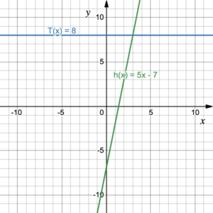
Figure 1. Constant function and linear function

When the highest exponent on a variable is at least 2, the graph is a curve. Figure 2 illustrates the graphs of the two polynomial functions [latex]\color{blue}{f(x)=x^2}[/latex] and [latex]\color{green}{f(x)=x^3}[/latex]. Notice that these functions are a completely different shape. However, they both pass through the points (0, 0) and (1, 1). All polynomial functions are continuous with a domain of [latex](-\infty, +\infty)[/latex], which means that the independent variable [latex]x[/latex] can take on any real number value.

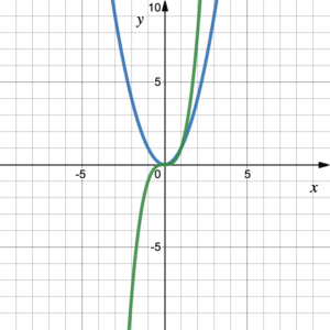
Figure 2. Polynomial functions

Example 1

Use the Desmos Graphing Calculator to determine the shape of the functions:

[latex]f(x)=x^4[/latex]

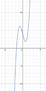
[latex]g(x)=x^3-4x^2+5x-2[/latex]

[latex]h(x)=x^6-2x^3+x[/latex]

Solution

Go to the Desmos Graphing Calculator and type each function into a box on the left side of the screen. Use the ^ (carat) key on your keyboard for exponents.

​

[latex]f(x)=x^4[/latex]

[latex]g(x)=x^3-4x^2+5x-2[/latex]

[latex]h(x)=x^6-2x^3+x[/latex]

Try It 1

Use the Desmos Graphing Calculator to determine the shape of the functions:

[latex]f(x)=x^5[/latex]

[latex]g(x)=3x-4[/latex]

[latex]h(x)=x^6-3x^3+2x-5[/latex]

Show Answer

​​

[latex]f(x)=x^5[/latex]

[latex]g(x)=3x-4[/latex]

[latex]h(x)=x^6-3x^3+2x-5[/latex]

Exponential Functions

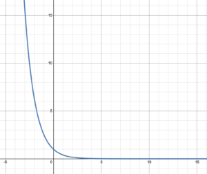
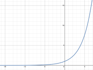
An exponential function is a function where the independent variable sits at the exponent position. The functions [latex]f(x)=4^x,\;g(x)=(3.2)^x, \;h(x)=\left (\frac{1}{5}\right )^x[/latex] are all examples of exponential functions: a positive real number raised to a power of [latex]x[/latex]. Figure 3 illustrates the graphs of four exponential functions: [latex]f(x)=2^x, \;g(x)=3^x, \;r(x)=5^x, s(x)=\;10^x[/latex]. Notice that each of these graphs have the same basic shape. They slowly come up from the [latex]x[/latex]-axis then quickly move towards [latex]+\infty[/latex].  The graphs never quite make it to the line [latex]y=0[/latex] (the [latex]x[/latex]-axis) and this line is referred to as a horizontal asymptote; a horizontal line that the graph never quite reaches as it moves towards either positive or negative (in this case) infinity. In addition, they all pass through the point (0, 1).

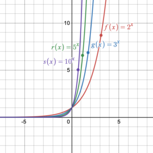
Figure 3. Exponential functions.

Example 2

Use the Desmos Graphing Calculator to determine the shape of the functions:

[latex]f(x)=4^x[/latex]

[latex]g(x)=\left (\frac{1}{4}\right )^x[/latex]

[latex]h(x)=(3.5)^x[/latex]

Solution

Go to the Desmos Graphing Calculator and type each function into a box on the left side of the screen.

[latex]f(x)=4^x[/latex]

[latex]g(x)=\left (\frac{1}{4}\right )^x[/latex]

[latex]h(x)=(3.5)^x[/latex]

Did you notice that the line [latex]y=0[/latex] is a horizontal asymptote for all of the graphs; that they all pass through (0, 1); and that they all pass through [latex](1, a)[/latex] where [latex]a[/latex] is the base? [latex]f(x)=4^x[/latex] passes through (1, 4); [latex]g(x)=\left (\frac{1}{4}\right )^x[/latex] passes through [latex](1, \frac{1}{4})[/latex]; and [latex]h(x)=(3.5)^x[/latex] passes through (1, 3.5).

What makes the graphs of[latex]f(x)=4^x[/latex] and [latex]h(x)=(3.5)^x[/latex] different from [latex]g(x)=\left (\frac{1}{4}\right )^x[/latex]? The first two are continuously increasing while the last is continuously decreasing. Why? When the base of the exponential expression is > 1 the graph will increase. When the base of the graph lies between 0 and 1, the graph will decrease.

What happens if we try a base of 0, 1 or a negative number?  Try it in Desmos and see!

Try It 2

Use the Desmos Graphing Calculator to determine the shape of the functions:

[latex]f(x)=7^x[/latex]

[latex]g(x)=\left (\frac{2}{5}\right )^x[/latex]

[latex]h(x)=(1.5)^x[/latex]

Show Answer

[latex]f(x)=7^x[/latex]

[latex]g(x)=\left (\frac{2}{5}\right )^x[/latex]

[latex]h(x)=(1.5)^x[/latex]

Logarithmic Functions

The inverse of an exponential function is referred to as a logarithmic function. If we were to find the inverse of each of the functions in figure 2 by reflecting them across the line [latex]y=x[/latex] we would get their inverse functions. Recall that to find an inverse function, all we do is switch the variables. So if we let [latex]y=f(x)[/latex] in the function [latex]f(x)=2^x[/latex], then [latex]y=2^x[/latex] and the inverse function is simply [latex]x=2^y[/latex]. Typically, we write an inverse function in function notation, which would require solving for [latex]y[/latex]. We will learn how to do this later in the course, but for now it will suffice to know that the notation for this inverse function requires the use of a logarithm. No one wants to write logarithm more than once, so we truncate it to log. To indicate the base of the exponent in the function where [latex]x=2^y[/latex], we write [latex]f(x)=log_2x[/latex]. This is read, “[latex]f[/latex] of [latex]x[/latex] equals log base 2 of [latex]x[/latex]. The base is always written as a subscript attached to log. A logarithm always has a base. Had the function been [latex]x=3^y[/latex] we would write [latex]g(x)=log_3x[/latex] and if the function was [latex]x=10^y[/latex] we would write [latex]h(x)=log_{10}x[/latex].

Figure 4 shows graphs of three logarithmic functions: [latex]f(x)=log_2 x, g(x)=log_3 x, s(x)=log_{10} x[/latex]. Notice that each of the graphs follows the same basic shape; coming up fast from [latex]y=-\infty[/latex] close to [latex]x=0[/latex] then slowly heading continuously upwards towards [latex]+\infty[/latex]. Notice also that each graph passes through the point (1, 0) and none of these graphs cross the [latex]y[/latex]-axis. In this case, the line [latex]x=0[/latex] (the [latex]y[/latex]-axis) is an example of a vertical asymptote; a vertical line that the graph never crosses.

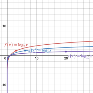
Figure 4. Logarithmic functions.

Example 3

Use the Desmos Graphing Calculator to determine the shape of the functions:

[latex]f(x)=log_{10}x[/latex]

[latex]g(x)=log_{\frac{1}{4}}x[/latex]

[latex]h(x)=log_8 x[/latex]

Solution

To type a subscript for the base of the log, use the underscore key (shift -). After you enter the base you must click past the base to insert [latex]x[/latex]. So [latex]f(x)=log_{10}x[/latex] will be typed in as f(x)=log_10 “click past 10 to get back to standard script” x

[latex]f(x)=log_{10}x[/latex]

[latex]g(x)=log_{\frac{1}{4}}x[/latex]

[latex]h(x)=log_8 x[/latex]

Did you notice that the line [latex]x=0[/latex] is a vertical asymptote for all of the graphs; that they all pass through (1, 0); and that they all pass through [latex](a, 1)[/latex] where [latex]a[/latex] is the base? [latex]f(x)=log_{10}x[/latex] passes through (10, 1); [latex]g(x)=log_{\frac{1}{4}} x[/latex] passes through [latex]\left ( \frac{1}{4}, 1\right )[/latex]; and [latex]h(x)=log_8 x[/latex] passes through (8, 1).

What makes the graphs of  [latex]f(x)=log_{10}x[/latex] and [latex]h(x)=log_8 x[/latex] different from [latex]g(x)=log_{\frac{1}{4}}x[/latex]? The first two are continuously increasing while the last is continuously decreasing. Why? When the base of the logarithm is > 1 the graph will increase. When the base of the graph lies between 0 and 1, the graph will decrease.

What happens if we try a base of 0, 1 or a negative number?  Try it in Desmos and see!

Try It 3

Use the Desmos Graphing Calculator to determine the shape of the functions:

[latex]f(x)=log_{12}x[/latex]

[latex]g(x)=log_{\frac{1}{8}}x[/latex]

[latex]h(x)=log_2 x[/latex]

Show Answer

[latex]f(x)=log_{12}x[/latex]

[latex]g(x)=log_{\frac{1}{8}}x[/latex]

[latex]h(x)=log_2 x[/latex]

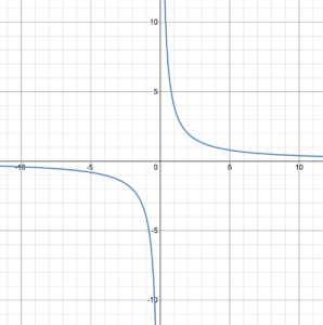
Rational Functions

A rational function is a function where the independent variable is in the denominator of a fraction. Technically it is one polynomial function divided by another polynomial function. It can be as basic as [latex]f(x)=\frac{1}{x}[/latex] or more complicated like [latex]g(x)=\frac{5x^5-3x^4+2x^3-x^2+6}{x^6-2x+8}[/latex]. Figure 5 shows the graphs of two basic rational functions. Later in this course we will go into more detail on these basic functions. The graphs of more complicated functions are shown in figures 6 and 7. Notice that the graphs of both functions in figure 5 have horizontal and vertical asymptotes. The graph of the function in figure 7 has only a horizontal asymptote, and the graph of the function in figure 6 has a vertical and a slant asymptote. If you take College Algebra, you will learn more about these asymptotes.

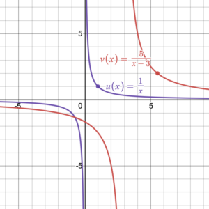
Figure 5. Rational functions.

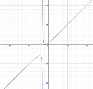
Figure 6. A rational function with vertical and slant asymptotes.

Figure 7. Rational function with a horizontal asymptote.

Example 4

Use the Desmos Graphing Calculator to determine the shape of the functions:

[latex]f(x)=\frac{1}{3x}[/latex]

[latex]g(x)=\frac{6}{x}[/latex]

[latex]h(x)=\frac{x^2}{x-3}[/latex]

Solution

To type a rational function into desmos, type “frac” and a fraction will appear. Type the numerator of the function, then click on the denominator and type the denominator of the function.

[latex]f(x)=\frac{1}{3x}[/latex]

[latex]g(x)=\frac{6}{x}[/latex]

[latex]h(x)=\frac{x^2}{x-3}[/latex]

Did you notice that the graphs of [latex]f(x)=\frac{1}{3x}[/latex] and [latex]g(x)=\frac{6}{x}[/latex] have a vertical asymptote and a horizontal asymptote? On the other hand, the graph of [latex]h(x)=\frac{x^2}{x-3}[/latex] has a vertical asymptote and a slant asymptote.

Try It 4

Use the Desmos Graphing Calculator to determine the shape of the functions:

[latex]f(x)=\frac{4}{x}[/latex]

[latex]g(x)=\frac{3}{8x}[/latex]

[latex]h(x)=\frac{x+4}{x^{2}-5x+6}[/latex]

Show Answer

[latex]f(x)=\frac{4}{x}[/latex]

[latex]g(x)=\frac{3}{8x}[/latex]

[latex]h(x)=\frac{x+4}{x^{2}-5x+6}[/latex]

Functions take on many shapes. A graphing calculator like Desmos helps us visualize the graphs of functions letting us see asymptotes, intercepts, turning points and other graphical features. In this section, we highlighted the types of graphs and functions we are going to look at in more detail in this course.

Try It 5

Identify the type of function from its graph.

Show Answer

1. Polynomial function
2. Logarithmic function
3. Exponential function