Learning Outcomes
- Use arrow notation to describe local and end behavior of rational functions.
- Identify horizontal and vertical asymptotes of rational functions from graphs.
- Graph a rational function given horizontal and vertical shifts.
- Solve applied problems involving rational functions.
Using Arrow Notation
recall Characteristics of rational expressions
- We’ve seen that rational expressions are fractions that may contain a polynomial in the numerator, denominator, or both.
- A rational function is a function whose argument is defined using a rational expression.
- When a variable is present in the denominator of a rational expression, certain values of the variable may cause the denominator to equal zero. A rational expression with a zero in the denominator is not defined since we cannot divide by zero.
- We’ll see in this section that the values of the input to a rational function causing the denominator to equal zero will have an impact on the shape of the function’s graph. The graph appears to “bend around” these input values, and the function value increases or decreases without bound near those inputs.
- See the graphs below for how to use a notation called arrow notation to describe this and other behaviors sometimes present in the graphs of functions.
We have seen the graphs of the basic reciprocal function and the squared reciprocal function from our study of toolkit functions. Examine these graphs and notice some of their features.
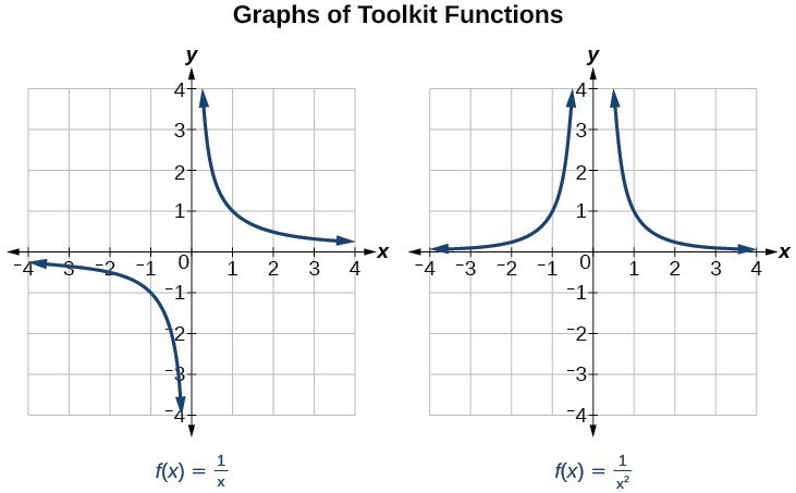
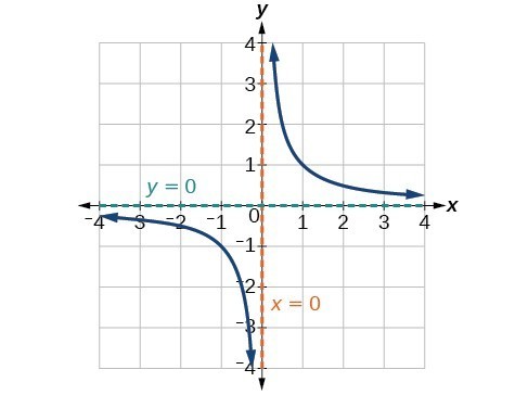
Several things are apparent if we examine the graph of [latex]f\left(x\right)=\dfrac{1}{x}[/latex].
- On the left branch of the graph, the curve approaches the [latex]x[/latex]-axis [latex]\left(y=0\right) \text{ as } x\to -\infty[/latex].
- As the graph approaches [latex]x=0[/latex] from the left, the curve drops, but as we approach zero from the right, the curve rises.
- Finally, on the right branch of the graph, the curves approaches the [latex]x[/latex]–axis [latex]\left(y=0\right) \text{ as } x\to \infty[/latex].
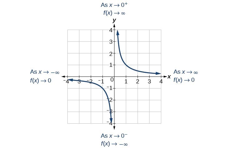
To summarize, we use arrow notation to show that [latex]x[/latex] or [latex]f\left(x\right)[/latex] is approaching a particular value.
| Arrow Notation | |
|---|---|
| Symbol | Meaning |
| [latex]x\to {a}^{-}[/latex] | [latex]x[/latex] approaches [latex]a[/latex] from the left ([latex]x\lt a[/latex] but close to [latex]a[/latex]) |
| [latex]x\to {a}^{+}[/latex] | [latex]x[/latex] approaches [latex]a[/latex] from the right ([latex]x\lt a[/latex] but close to [latex]a[/latex]) |
| [latex]x\to \infty[/latex] | [latex]x[/latex] approaches infinity ([latex]x[/latex] increases without bound) |
| [latex]x\to -\infty[/latex] | [latex]x[/latex] approaches negative infinity ([latex]x[/latex] decreases without bound) |
| [latex]f\left(x\right)\to \infty[/latex] | the output approaches infinity (the output increases without bound) |
| [latex]f\left(x\right)\to -\infty[/latex] | the output approaches negative infinity (the output decreases without bound) |
| [latex]f\left(x\right)\to a[/latex] | the output approaches [latex]a[/latex] |
Local Behavior of [latex]f\left(x\right)=\frac{1}{x}[/latex]
Let’s begin by looking at the reciprocal function, [latex]f\left(x\right)=\frac{1}{x}[/latex]. We cannot divide by zero, which means the function is undefined at [latex]x=0[/latex]; so zero is not in the domain.
As the input values approach zero from the left side (becoming very small, negative values), the function values decrease without bound (in other words, they approach negative infinity). We can see this behavior in the table below.
| [latex]x[/latex] | –0.1 | –0.01 | –0.001 | –0.0001 |
| [latex]f\left(x\right)=\frac{1}{x}[/latex] | –10 | –100 | –1000 | –10,000 |
We write in arrow notation:
[latex]\text{as }x\to {0}^{-},f\left(x\right)\to -\infty[/latex]
As [latex]x[/latex] approaches [latex]0[/latex] from the left (negative) side, [latex]f(x)[/latex] will approach negative infinity.
As the input values approach zero from the right side (becoming very small, positive values), the function values increase without bound (approaching infinity). We can see this behavior in the table below.
| [latex]x[/latex] | 0.1 | 0.01 | 0.001 | 0.0001 |
| [latex]f\left(x\right)=\frac{1}{x}[/latex] | 10 | 100 | 1000 | 10,000 |
We write in arrow notation:
[latex]\text{As }x\to {0}^{+}, f\left(x\right)\to \infty[/latex].
As [latex]x[/latex] approaches [latex]0[/latex] from the right (positive) side, [latex]f(x)[/latex] will approach infinity.
This behavior creates a vertical asymptote, which is a vertical line that the graph approaches but never crosses. In this case, as the input nears zero from the left, the function value decreases without bound. As the input nears zero from the right, the function value increases without bound. The line [latex]x=0[/latex] is a vertical asymptote for the function.
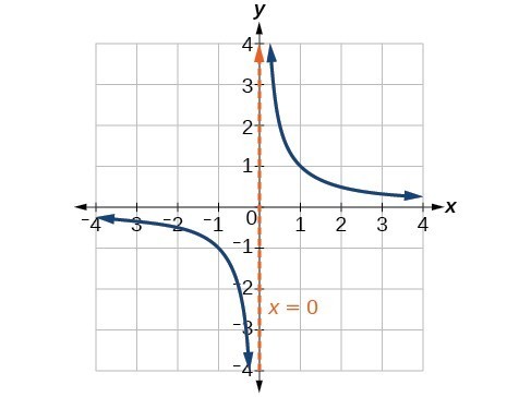
A General Note: Vertical Asymptote
A vertical asymptote of a graph is a vertical line [latex]x=a[/latex] where the graph tends toward positive or negative infinity as the inputs approach [latex]x[/latex]. We write
[latex]\text{As }x\to a,f\left(x\right)\to \infty , \text{or as }x\to a,f\left(x\right)\to -\infty[/latex].
Asymptote. what does that word mean?
The term asymptote has its origins from three Greek roots.
a, meaning not
sun, meaning together
ptotos, meaning to fall
These give us asymptotos, meaning not falling together, which leads to the modern term describing a line that a curve (the graph of a function) approaches but never meets.
End Behavior of [latex]f\left(x\right)=\frac{1}{x}[/latex]
As the values of [latex]x[/latex] approach infinity, the function values approach 0. As the values of [latex]x[/latex] approach negative infinity, the function values approach 0. Symbolically, using arrow notation
[latex]\text{As }x\to \infty ,f\left(x\right)\to 0,\text{and as }x\to -\infty ,f\left(x\right)\to 0[/latex].
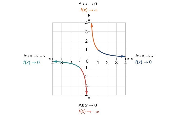
Based on this overall behavior and the graph, we can see that the function approaches 0 but never actually reaches 0; it seems to level off as the inputs become large. This behavior creates a horizontal asymptote, a horizontal line that the graph approaches as the input increases or decreases without bound. In this case, the graph is approaching the horizontal line [latex]y=0[/latex].
A General Note: Horizontal Asymptote
A horizontal asymptote of a graph is a horizontal line [latex]y=b[/latex] where the graph approaches the line as the inputs increase or decrease without bound. We write
[latex]\text{As }x\to \infty \text{ or }x\to -\infty ,\text{ }f\left(x\right)\to b[/latex].
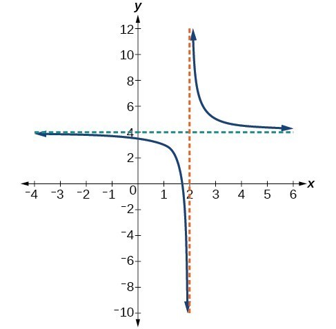
Example: Using Arrow Notation
Use arrow notation to describe the end behavior and local behavior of the function below.
Try It
Use arrow notation to describe the end behavior and local behavior for the reciprocal squared function.
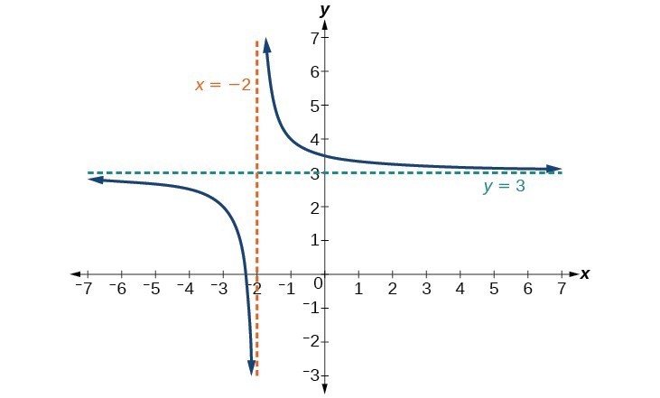
Example: Using Transformations to Graph a Rational Function
Sketch a graph of the reciprocal function shifted two units to the left and up three units. Identify the horizontal and vertical asymptotes of the graph, if any.
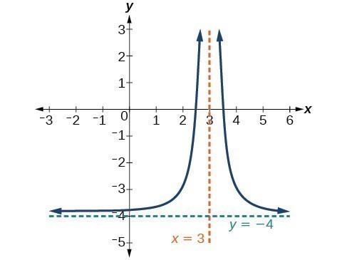
Try It
Sketch the graph, and find the horizontal and vertical asymptotes of the reciprocal squared function that has been shifted right 3 units and down 4 units.
Solve Applied Problems Involving Rational Functions
In the previous example, we shifted a toolkit function in a way that resulted in the function [latex]f\left(x\right)=\dfrac{3x+7}{x+2}[/latex]. This is an example of a rational function. A rational function is a function that can be written as the quotient of two polynomial functions. Many real-world problems require us to find the ratio of two polynomial functions. Problems involving rates and concentrations often involve rational functions.
A General Note: Rational Function
A rational function is a function that can be written as the quotient of two polynomial functions [latex]P\left(x\right) \text{and} Q\left(x\right)[/latex].
[latex]f\left(x\right)=\dfrac{P\left(x\right)}{Q\left(x\right)}=\dfrac{{a}_{p}{x}^{p}+{a}_{p - 1}{x}^{p - 1}+...+{a}_{1}x+{a}_{0}}{{b}_{q}{x}^{q}+{b}_{q - 1}{x}^{q - 1}+...+{b}_{1}x+{b}_{0}},Q\left(x\right)\ne 0[/latex]
Summary: Horizontal and Vertical asymptotes
Horizontal Asymptote
- A horizontal line of the form [latex]y=c[/latex]
- The constant [latex]c[/latex] represents a number that the function value (output) approaches in the long run, either as the input grows very small or very large.
- Horizontal asymptotes represent the long-run behavior (the end behavior) of the graph of the function.
- A function’s graph may cross a horizontal asymptote briefly, even more than once, but will eventually settle down near it, as the value of the function approaches the constant [latex]c[/latex].
Vertical Asymptote
- A vertical line of the form [latex]x=a[/latex]
- The constant [latex]a[/latex] represents an input for which the function value (output) is undefined.
- Substituting the value of [latex]a[/latex] into the function will result in a zero in the function’s denominator.
- The graph of the function “bends around”, either increasing or decreasing without bound as the input nears [latex]a[/latex]
- A function’s graph will never cross a vertical asymptote.
Example: Solving an Applied Problem Involving a Rational Function
A large mixing tank currently contains 100 gallons of water into which 5 pounds of sugar have been mixed. A tap will open pouring 10 gallons per minute of water into the tank at the same time sugar is poured into the tank at a rate of 1 pound per minute. Find the concentration (pounds per gallon) of sugar in the tank after 12 minutes. Is that a greater concentration than at the beginning?
Try It
There are 1,200 freshmen and 1,500 sophomores at a prep rally at noon. After 12 p.m., 20 freshmen arrive at the rally every five minutes while 15 sophomores leave the rally. Find the ratio of freshmen to sophomores at 1 p.m.
Candela Citations
- Revision and Adaptation. Provided by: Lumen Learning. License: CC BY: Attribution
- Question ID 129042, 129067. Authored by: Day, Alyson. License: CC BY: Attribution. License Terms: IMathAS Community License CC-BY + GPL
- College Algebra. Authored by: Abramson, Jay et al.. Provided by: OpenStax. Located at: http://cnx.org/contents/9b08c294-057f-4201-9f48-5d6ad992740d@5.2. License: CC BY: Attribution. License Terms: Download for free at http://cnx.org/contents/9b08c294-057f-4201-9f48-5d6ad992740d@5.2