Why Study Algebraic Operations on Functions?
If you could “see” the sound coming from your speakers or earphones, it might resemble a series of ups and downs corresponding to the vibrations caused by the sound as it travels through the air. In fact, with the help of a tool called an oscilloscope, it is possible to visualize sounds as waves (technically, sound travels through air as a series of compression waves, however the oscilloscope converts sound to transverse waves for better visualization).
The wave itself may be regarded as the graph of a function. In other words, the sound wave may be modeled by the rule
[latex]y=f\left(x\right)[/latex]
It is not essential to understand exactly how this function is put together – you might learn more about the details of sound waves after studying a little trigonometry – however we can use what we learn in this module to transform the wave in certain ways.
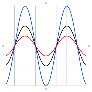
Figure 1
For example, if we made the sound louder (increasing the amplitude), then the oscilloscope would display the same basic wave graph but with higher peaks and deeper valleys. The new function is a vertical stretch of the original.
Conversely, if we made the sound softer (decreasing the amplitude), then the new wave would have lower peaks and shallower valleys, which is a vertical compression.
Figure 1 illustrates how the graph of a function in black might stretch vertically into the blue curve, or compress vertically into the red curve. What is the effect on the original function? It turns out that vertical compression and stretching can be accomplished by multiplying or dividing the output of the function by a constant ([latex]a[/latex]):
[latex]y=a\cdot f\left(x\right)[/latex]
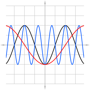
Figure 2
Some sounds, such as musical tones, also have pitch, or a measure of how high or how low the tone sounds. If run your finger along the keys of a piano from left to right, the tones increase steadily in pitch. Pitch is measured by the frequency of a wave, which is the number of peaks within a given time period. Frequency is easy to see on the oscilloscope: the more wave peaks you see on the screen, the higher the frequency, and the higher the pitch of the sound.
To change the frequency of the wave we must stretch or compress the graph horizontally. Figure 2 illustrates the effect of horizontal compression (blue curve) and stretching (red curve) of the original curve (in black). If the black curve represents a musical tone, then the blue curve will sound higher, while the red curve will sound lower in pitch. Horizontal stretching and compression is handled by multiplying (or dividing) a constant to the input [latex]x[/latex]:
[latex]y=f\left(b\cdot x\right)[/latex]
In this module, you will learn all about these kinds of transformations along with other ways of changing and combining functions.
Candela Citations
- Why It Matters: Algebraic Operations on Functions. Authored by: Lumen Learning. License: CC BY: Attribution
- 3 sinusoidal waves (Figure 1). Authored by: Shaun Ault for Lumen. License: CC BY: Attribution
- 3 sinusoidal waves (Figure 2). Authored by: Shaun Ault for Lumen. License: CC BY: Attribution
- Revision and Adaptation. Provided by: Lumen Learning. License: CC BY: Attribution
- Tektronix Oscilloscope. Authored by: stanhua. Located at: https://www.flickr.com/photos/stanhua/149924240. License: CC BY: Attribution