Learning Outcomes
- Evaluate and rewrite logarithms using the properties of logarithms
- Use the properties of logarithms to solve exponential models for time
- Identify the carrying capacity in a logistic growth model
- Use a logistic growth model to predict growth
Limits on Exponential Growth
In our basic exponential growth scenario, we had a recursive equation of the form
Pn = Pn-1 + r Pn-1
In a confined environment, however, the growth rate may not remain constant. In a lake, for example, there is some maximum sustainable population of fish, also called a carrying capacity.
Carrying Capacity
The carrying capacity, or maximum sustainable population, is the largest population that an environment can support.

For our fish, the carrying capacity is the largest population that the resources in the lake can sustain. If the population in the lake is far below the carrying capacity, then we would expect the population to grow essentially exponentially. However, as the population approaches the carrying capacity, there will be a scarcity of food and space available, and the growth rate will decrease. If the population exceeds the carrying capacity, there won’t be enough resources to sustain all the fish and there will be a negative growth rate, causing the population to decrease back to the carrying capacity.
If the carrying capacity was 5000, the growth rate might vary something like that in the graph shown.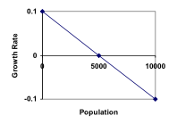
Note that this is a linear equation with intercept at 0.1 and slope [latex]-\frac{0.1}{5000}[/latex], so we could write an equation for this adjusted growth rate as:
radjusted = [latex]0.1-\frac{0.1}{5000}P=0.1\left(1-\frac{P}{5000}\right)[/latex]
Substituting this in to our original exponential growth model for r gives
[latex]{{P}_{n}}={{P}_{n-1}}+0.1\left(1-\frac{{{P}_{n-1}}}{5000}\right){{P}_{n-1}}[/latex]
View the following for a detailed explanation of the concept.
Logistic Growth
If a population is growing in a constrained environment with carrying capacity K, and absent constraint would grow exponentially with growth rate r, then the population behavior can be described by the logistic growth model:
[latex]{{P}_{n}}={{P}_{n-1}}+r\left(1-\frac{{{P}_{n-1}}}{K}\right){{P}_{n-1}}[/latex]
Unlike linear and exponential growth, logistic growth behaves differently if the populations grow steadily throughout the year or if they have one breeding time per year. The recursive formula provided above models generational growth, where there is one breeding time per year (or, at least a finite number); there is no explicit formula for this type of logistic growth.
Examples
A forest is currently home to a population of 200 rabbits. The forest is estimated to be able to sustain a population of 2000 rabbits. Absent any restrictions, the rabbits would grow by 50% per year. Predict the future population using the logistic growth model.
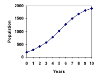
View more about this example below.
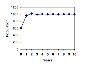
On an island that can support a population of 1000 lizards, there is currently a population of 600. These lizards have a lot of offspring and not a lot of natural predators, so have very high growth rate, around 150%. Calculating out the next couple generations:
[latex]{{P}_{1}}={{P}_{0}}+1.50\left(1-\frac{{{P}_{0}}}{1000}\right){{P}_{0}}=600+1.50\left(1-\frac{600}{1000}\right)600=960[/latex]
[latex]{{P}_{2}}={{P}_{1}}+1.50\left(1-\frac{{{P}_{1}}}{1000}\right){{P}_{1}}=960+1.50\left(1-\frac{960}{1000}\right)960=1018[/latex]
Interestingly, even though the factor that limits the growth rate slowed the growth a lot, the population still overshot the carrying capacity. We would expect the population to decline the next year.
[latex]{{P}_{3}}={{P}_{2}}+1.50\left(1-\frac{{{P}_{3}}}{1000}\right){{P}_{3}}=1018+1.50\left(1-\frac{1018}{1000}\right)1018=991[/latex]
Calculating out a few more years and plotting the results, we see the population wavers above and below the carrying capacity, but eventually settles down, leaving a steady population near the carrying capacity.
Try It
A field currently contains 20 mint plants. Absent constraints, the number of plants would increase by 70% each year, but the field can only support a maximum population of 300 plants. Use the logistic model to predict the population in the next three years.
Example
On a neighboring island to the one from the previous example, there is another population of lizards, but the growth rate is even higher – about 205%.
Calculating out several generations and plotting the results, we get a surprise: the population seems to be oscillating between two values, a pattern called a 2-cycle.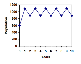
While it would be tempting to treat this only as a strange side effect of mathematics, this has actually been observed in nature. Researchers from the University of California observed a stable 2-cycle in a lizard population in California.[1]
Taking this even further, we get more and more extreme behaviors as the growth rate increases higher. It is possible to get stable 4-cycles, 8-cycles, and higher. Quickly, though, the behavior approaches chaos (remember the movie Jurassic Park?).

All of the lizard island examples are discussed in this video.
Try It
Candela Citations
- Revision and Adaptation. Provided by: Lumen Learning. License: CC BY: Attribution
- Logistic Growth. Authored by: David Lippman. Located at: http://www.opentextbookstore.com/mathinsociety/. Project: Math in Society. License: CC BY-SA: Attribution-ShareAlike
- fishes-colourful-beautiful-koi. Authored by: sharonang. Located at: https://pixabay.com/en/fishes-colourful-beautiful-koi-1711002/. License: CC0: No Rights Reserved
- Logistic model. Authored by: OCLPhase2's channel. Located at: https://youtu.be/-6VLXCTkP_c. License: CC BY: Attribution
- Logistic growth of rabbits. Authored by: OCLPhase2's channel. Located at: https://youtu.be/dPOlEgJ2QX0. License: CC BY: Attribution
- Logistic growth of lizards. Authored by: OCLPhase2's channel. Located at: https://youtu.be/fuJF_uZGoFc. License: CC BY: Attribution
- Question ID 54627. Authored by: Hartley,Josiah. License: CC BY: Attribution. License Terms: IMathAS Community License
- Question ID 6589. Authored by: Lippman,David. License: CC BY: Attribution. License Terms: IMathAS Community License CC-BY + GPL