Learning Outcomes
- Use logical functions and formulas
Excel logic functions evaluate whether the statement and data are considered true or false according to how the formula is established. We will cover the top used Excel logical functions in this section. Exactly like the financial functions, you can use the Formulas tab as before to insert the function or you can begin by typing an equal sign in a cell.
Nested IF
Taking an IF function and adding more than one logic test inside the IF function. In other words, start with and IF function and add another IF function inside the original IF function. A Nested IF formula looks like this: =IF(logical_test,[value_if_true],[value_if_false],IF(logical_test,[value_if_true],[value_if_false]))
Previously, you learned how to use the IF function as a logical way to test your data. Let’s consider that we want to see two variables run at once to create a logical outcome. We’ll now look at Regional Sales for five salespeople over a year and see if they meet the requirements for an annual commission and what the commission amount would be.
Note
Two shortcuts for locking down a cell to make it absolute instead of relative. You’ll need to know these to work faster through creating formulas.
- Short cut key F4 automatically adds in $ to a cell location information to lock it down and make it absolute to stop it from changing as it is dragged into other cells or ranges (e.g. $D$3).
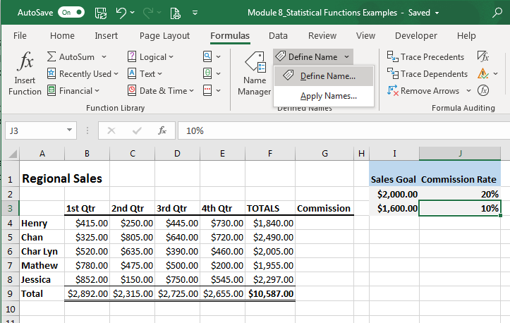
- Name Range locks down a cell like $. To create a Name Range, highlight the cell, click on the Formulas tab, Define Name button. After the dialog box opens, name the location (no spaces) to make it unique for navigation or for formulas (e.g. Commission_Rate).
With a sales spreadsheet open, look at the tiered commission structure. There are two possibilities to earn commission. A Nested IF function is a perfect formula to calculate which salesperson receives how much commission.
Follow these steps to create a Nested IF function:
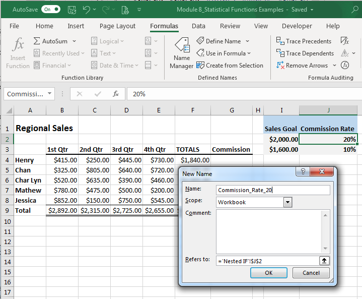
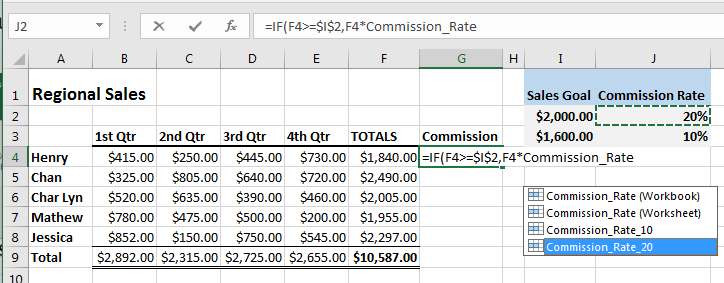
- First let’s define names for the two types of commissions as this will make it easier to distinguish in the formula. Select the 20% cell and click on the Formula tab, Define Name button and name it Commission_Rate_20. Follow the same steps to name the 10% commission cell too.
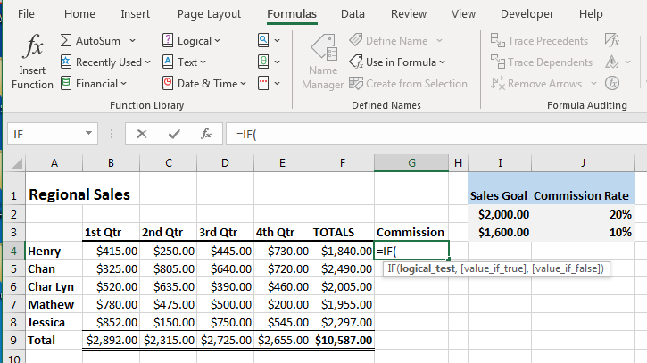
- Select the first cell under the commission heading and begin typing =IF, then hit the Tab key and a bracket will automatically appear displaying the logic formula for an IF function.
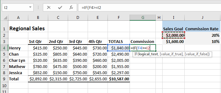
- Select the total sales for Henry (G4) and type in whether the total sales is less than or equal to the sales goal (G4>=I2). Be sure to hit the F4 button and the absolute $ will fill I2 so it will not change in any way if the formula is moved ($I$2), then type a comma.
- The next portion of the formula is for the percentage of commission to be paid if the goal has been reached. After the comma, choose the sales total again (F4) multiplied by the commission percentage by selecting the name you created earlier (F4*Commession_Rate_20), then a comma to separate the next part of the formula.
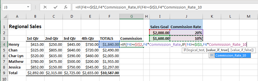
- The next portion of the formula is for the other percentage of commission to be paid if that lower goal has been met. After the comma, type another IF and hit the Tab key. Create the same formula again but use the Commission_Rate_10 this time and at the end a comma.
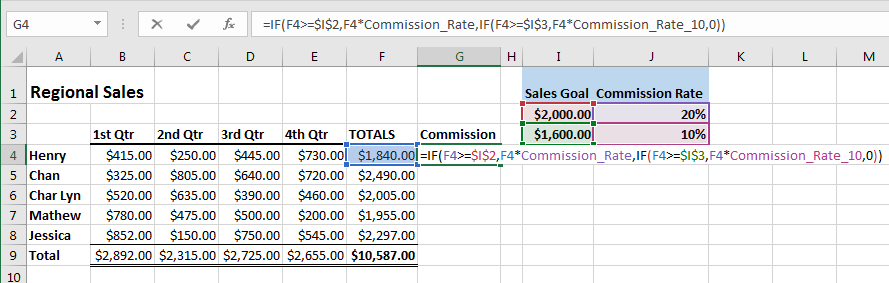
- The last portion of the formula is asking what to do if the logic comes back as a false answer. In this case, it will return a 0. Now finish with two end parentheses, one turns red indicating the second IF function, and then an additional end parenthesis to enclose the entire function begun with the first IF function.
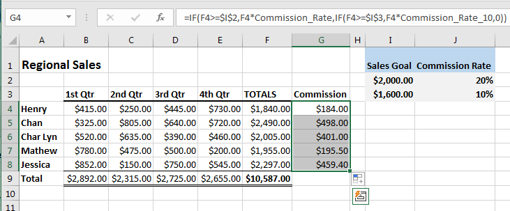
- Now copy the formula down the column all the way to the last salesperson’s total. These are the commissions paid based on the Nested IF formulas created. A nice logical function to make a more difficult task easier in a spreadsheet.
AND
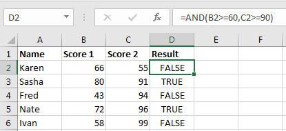
This function returns TRUE if all the arguments in its formula are TRUE and returns FALSE if any of the conditions are false. The Excel formula for this is =AND(logical1,[logical2],…).
In this example the AND function returns TRUE if the first score is greater than or equal to 60 and the second score is greater than or equal to 90, otherwise it returns FALSE.
OR
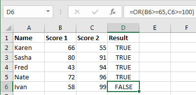
The OR function returns TRUE if any of the arguments are TRUE. The Excel formula for this is =OR(logical1,[logical2],…).
In this example the AND function returns TRUE if the first score is greater than or equal to 65 and the second score is greater than or equal to 100, otherwise it returns FALSE.
IFERROR
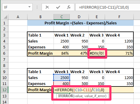
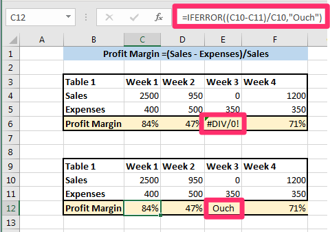
If your formula errors out, you can add in a value you specify how you would like it displayed. This logic function is beneficial to use if you occasionally run into errors and wish to have a cleaner looking spreadsheet to present.
The Excel formula for this is =IFERROR(value,value_if_error).
In this example there is an error in the Profit Margin row that is displayed at #DIV/0!. By using the IFERROR function an error like this can be displayed as a zero or even as text like “Ouch” if so desired. Here is what it looks like:
Practice Question
Candela Citations
- Logical Functions and Formulas. Authored by: Sherri Pendleton. Provided by: Lumen Learning. License: CC BY: Attribution
