Learning outcomes
- Conduct a chi-square test of independence. Interpret the conclusion in context.
Here we continue our chi-square test of independence for the variables gender and body image in the population of U.S. college students.
Example
Gender and Body Image Continued
Step 1: State the hypotheses.
Here are our hypotheses from the previous page:
- H0: There is no relationship between gender and body image for U.S. college students. (The variables are independent.)
- Ha: There is a relationship between gender and body image for U.S. college students. (The variables are dependent.)
Step 2: Collect and analyze the data.
If the variables are independent, the percentage of males and females with a given response will be the same or at least close. Previously, we determined that in our sample, there are differences in the percentage of males and females who answer “about right,” “overweight,” or “underweight.”
| Conditional Percents | ||||
|---|---|---|---|---|
| About right | Overweight | Underweight | Row Totals | |
| Female | 560/760 = 73.68% | 163/760 = 21.45% | 37/760 = 4.87% | 760/760 = 100% |
| Male | 295/440 = 67.00% | 72/440 = 16.36% | 73/440 = 16.59% | 440/440 = 100% |
| Column Totals | 855/1200 = 71.25% | 235/1200 = 19.58% | 110/1200 = 9.17% | 1200/1200 = 100% |
We need to determine if these differences are typical in random samples from a population where gender and body image are independent. Perhaps the differences we see in this sample are just fluctuations expected in random sampling. Or perhaps these differences are too large to be explained by chance. We will not know until we complete the hypothesis test.
Step 3: Assess the evidence.
We need to determine the expected values and the chi-square test statistic so that we can find the P-value.
Calculating Expected Values for a Test of Independence
Expected counts always describe what we expect to see in a sample if the null hypothesis is true. In this situation, if gender and body image are independent, then we expect the probability that a student answers “about right” in the sample to be the same probability that a male (or a female) student answers “about right” (similarly for “overweight” or “underweight” responses).
Here are the calculations of expected counts for the response “about right”:
- Probability that a student will answer “about right”: P(about right) = (855/1,200) = 0.7125
- Expected count of females in the sample who will answer “about right”: 0.7125(760) = 541.5
- Expected count of males in the sample who will answer “about right”: 0.7125(440) = 313.5
| Expected Counts | ||||
|---|---|---|---|---|
| About right | Overweight | Underweight | Row Totals | |
| Female | 541.5 | 148.8 | 760 | |
| Male | 313.5 | 86.2 | 440 | |
| Column Totals | 855 | 235 | 110 | 1200 |
Here are the calculations of expected counts for the response “overweight”:
- Probability that a student will answer “overweight”: P(overweight) = (235/1,200) = 0.1958
- Expected count of females in the sample who will answer “overweight”: 0.1958(760) = 148.8
- Expected count of males in the sample who will answer “overweight”: 0.1958(440) = 86.2
Try It
Recall the study of New York firefighters. Our null hypothesis says that participation in 9/11 rescue operations is not associated with alcohol-related problems for New York firefighters. (Alcohol-related problems and participation in 9/11 rescue are independent.)
| No risk for alcohol problems | Moderate to severe risk for alcohol problems | ||
|---|---|---|---|
| Participated in 9/11 rescue | 793 | 309 | 1102 |
| Did not participate in 9/11 rescue | 441 | 110 | 551 |
| 1234 | 419 | 1653 |
Try It
| Observed Counts | ||||
|---|---|---|---|---|
| About right | Overweight | Underweight | Row Totals | |
| Female | 560 | 163 | 37 | 760 |
| Male | 295 | 72 | 73 | 440 |
| Column Totals | 855 | 235 | 110 | 1200 |
Example
More on Gender and Body Image
Checking Conditions
The conditions for use of the chi-square distribution are the same as we learned previously:
- The sample is random.
- All of the expected counts are 5 or greater.
Since the data meets the conditions, we can proceed with calculating χ2 test statistic.
Calculating the Chi-Square Test Statistic
We calculate the chi-square test statistic as we did in “Chi-Square Test for One-Way Tables.”
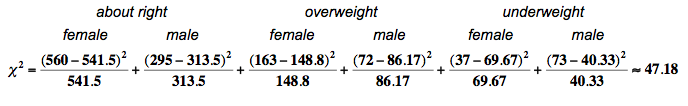
[latex]{\chi }^{2}\text{}=\text{}∑\frac{{(\mathrm{observed}-\mathrm{expected})}^{2}}{\mathrm{expected}}[/latex]
We will use technology to calculate the chi-square value. But for this sample, we will show the calculation.
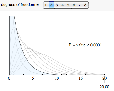
Finding Degrees of Freedom and the P-Value
For a chi-square tests based on two-way tables, the degrees of freedom are
- (number of explanatory categories – 1) × (number of response categories – 1)
You will also see this written: (r − 1)(c − 1), where r is the number of rows and c is the number of columns in the two-way table (when we write the table without row and column totals). In this case the degrees of freedom are (2 − 1)(3 −1 ) = 2.
We use the chi-square distribution with df = 2 to find the P-value. Note that the chi-square test statistic for this sample is so large that it is off the scale used in the simulation. So we conclude that the P-value is essentially zero.
Step 4: Conclusion
The relationship between gender and body image is statistically significant in this sample. We reject the null hypothesis and accept the alternative hypothesis. Gender and body image are dependent variables in the population of U.S. college students. (P-value is essentially 0.)
Try It
More on Gender and Body Piercing
A study was done on the relationship between gender and ear piercing among high-school students. A sample of 1,000 students was chosen, then classified according to both gender and whether or not they had either of their ears pierced. The following information is available:
| Chi-Square Test: Pierced, No Pierced | |||
|---|---|---|---|
| Observed Counts: | |||
| Pierced | No Pierced | Total | |
| Female | 576 | 64 | 640 |
| Male | 72 | 288 | 360 |
| Total | 648 | 352 | 1000 |
| Expected Counts: | |||
| Pierced | No Pierced | Total | |
| Female | 414.72 | 225.28 | 640 |
| Male | 233.28 | 126.72 | 360 |
| Total | 648 | 352 | 1000 |
| Chi-Square Contribution: | |||
| Pierced | No Pierced | ||
| Female | 115.462 | ||
| Male | 111.502 | 205.265 | |
Contribute!
Candela Citations
- Concepts in Statistics. Provided by: Open Learning Initiative. Located at: http://oli.cmu.edu. License: CC BY: Attribution