Learning OUTCOMES
- Use an exponential model (when appropriate) to describe the relationship between two quantitative variables. Interpret the model in context.
In our first example of exponential relationships, we investigate a nonlinear model for growth in a population over time.
Example
The Return of the Bald Eagle
During the mid-20th century, the population of bald eagles in the lower 48 states declined substantially. A highly toxic pesticide, DDT, was the main cause of the decline. DDT causes damage to bird egg shells. By 1963, bald eagles were in danger of complete extinction. Only 417 pairs of bald eagles remained. In 1967, the bald eagle became an official endangered species. Then in 1972, the EPA banned the use of DDT in the United States. The impact of the ban was a dramatic turnaround in the fate of the bald eagle.
Here is the data. Note that in the table, we defined t, our explanatory variable, to be Years after 1950. The response variable is the number of bald eagle pairs that are mating.
| Year | t = years after 1950 | Eagle Pairs |
|---|---|---|
| 1963 | 13 | 417 |
| 1974 | 24 | 791 |
| 1981 | 31 | 1188 |
| 1982 | 32 | 1480 |
| 1984 | 34 | 1757 |
| 1986 | 36 | 1875 |
| 1987 | 37 | 2238 |
| 1988 | 38 | 2475 |
| 1989 | 39 | 2680 |
| 1990 | 40 | 3035 |
| 1991 | 41 | 3399 |
| 1992 | 42 | 3749 |
| 1993 | 43 | 4015 |
| 1994 | 44 | 4449 |
| 1995 | 45 | 4712 |
| 1996 | 46 | 5094 |
| 1997 | 47 | 5295 |
| 1998 | 48 | 5748 |
| 1999 | 49 | 6104 |
| 2000 | 50 | 6471 |
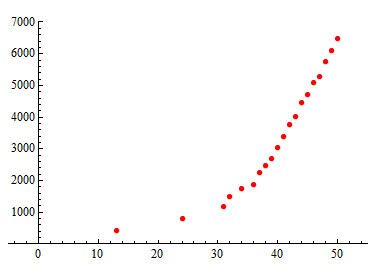
Our goal is to find an equation to model this relationship.
Here is a scatterplot of the data. We can see that the relationship appears somewhat linear, particularly for years after 1980 (t = 30). The correlation coefficient for this data set is high, r = 0.914.
The least squares regression line is Predicted eagle pairs = −3,878.11 + 185.4t. Below is a scatterplot of the data with the least-squares regression line and the residual plot.
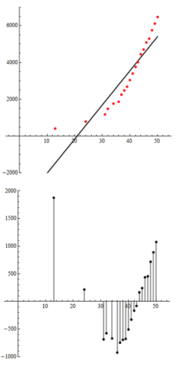
We see a clear pattern in the residuals, suggesting that a linear model does not capture patterns in the data.
Note: This is a reminder that a large r-value does not guarantee that a linear model is a good fit.
Conclusion: The data set for eagle pairs is clearly nonlinear. We need a better model.
In the scatterplot below, we fit an exponential model to the data. Notice how well this model describes the relationship between the variables. There is very little scatter about the exponential curve. There is a strong, positive exponential relationship between these variables.
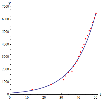
The equation of the exponential model is Predicted eagle pairs = 121 (1.083)t.
Note: In this equation, the t-variable is an exponent. Sometimes you will see this written with the caret symbol: ^. So Predicted y = 121 (1.083)t and Predicted y = 121(1.083) ^ t mean the same thing.
Now we use the exponential model to make predictions about the number of bald eagle mating pairs. We also compare the predictions from the exponential model to the linear model. Because there is a strong exponential relationship and a weaker linear relationship in the data, we expect the predictions from the exponential model to be better.
In 1963 (t = 13), there were 417 mating pairs.
- According to the linear model: Predicted eagle pairs = –3,878.11 + 185.4 (13) = (–1,468). Obviously, a negative value does not make sense for a count of eagle pairs.
- According to the exponential model: Predicted eagle pairs = 121 (1.083)13 = 341. So the exponential model underestimates by 417 – 341 = 76 mating pairs. But this is a much better prediction than we got from the linear model.
In 2000 (t = 50), there were 6,471 mating pairs.
- According to the linear model: Predicted eagle pairs = –3,878.11 + 185.4 (50) = 5,392. So the linear model underestimates by 6,471 – 5392 = 1,079 mating pairs.
- According to the exponential model: Predicted eagle pairs = 121 (1.083)50 = 6,519. So the exponential model overestimates by 6,591 – 6,471 = 48 mating pairs. This is a much better prediction than we got from the linear model.
Try It
Contribute!
Candela Citations
- Concepts in Statistics. Provided by: Open Learning Initiative. Located at: http://oli.cmu.edu. License: CC BY: Attribution