We learn a lot about things by seeing their pictorial representations, and that is exactly why graphing exponential equations is a powerful tool. It gives us another layer of insight for predicting future events. Before we begin graphing, it is helpful to review the behavior of exponential growth. Recall the table of values for a function of the form [latex]f\left(x\right)={b}^{x}[/latex] whose base is greater than one. We will use the function [latex]f\left(x\right)={2}^{x}[/latex]. Observe how the output values in the table below change as the input increases by [latex]1[/latex].

Each output value is the product of the previous output and the base, [latex]2[/latex]. We call the base [latex]2[/latex] the constant ratio. In fact, for any exponential function of the form [latex]f\left(x\right)=a{b}^{x},[/latex] b is the constant ratio of the function. This means that as the input increases by [latex]1[/latex], the output value will be the product of the base and the previous output, regardless of the value of a.

Notice from the table that

• the output values are positive for all values of x;
• as x increases, the output values increase without bound; and
• as x decreases, the output values grow smaller, approaching zero.

As x decreases, the output values grow smaller and smaller, getting closer and closer to zero but never actually reaching zero or crossing the x-axis.  This is a special property of this type of graph.  We say that the x-axis is an asymptote of an exponential growth function.

The graph below shows the exponential growth function [latex]f\left(x\right)={2}^{x}[/latex].

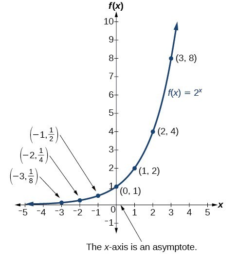
In the graph, notice that the graph gets close to the x-axis, but never touches it.

The domain of [latex]f\left(x\right)={2}^{x}[/latex] is all real numbers; the range is [latex]\left(0,\infty \right)[/latex].

To get a sense of the behavior of exponential decay, we can create a table of values for a function of the form [latex]f\left(x\right)={b}^{x}[/latex] whose base is between zero and one. We will use the function [latex]g\left(x\right)={\left(\frac{1}{2}\right)}^{x}[/latex]. Observe how the output values in the table below change as the input increases by [latex]1[/latex].

Again, because the input is increasing by [latex]1[/latex], each output value is the product of the previous output and the base, or constant ratio [latex]\frac{1}{2}[/latex].

Notice from the table that:

• the output values are positive for all values of x;
• as x increases, the output values grow smaller, approaching zero; and
• as x decreases, the output values grow without bound.

Similar to the exponential growth functions, a special property of exponential decay functions is that as the input values get larger and larger, the output values get closer and closer to zero without every actually touching or crossing the x-axis.  As a result, we say that the x-axis is an asymptote of an exponential decay function.

The graph shows the exponential decay function, [latex]g\left(x\right)={\left(\frac{1}{2}\right)}^{x}[/latex].

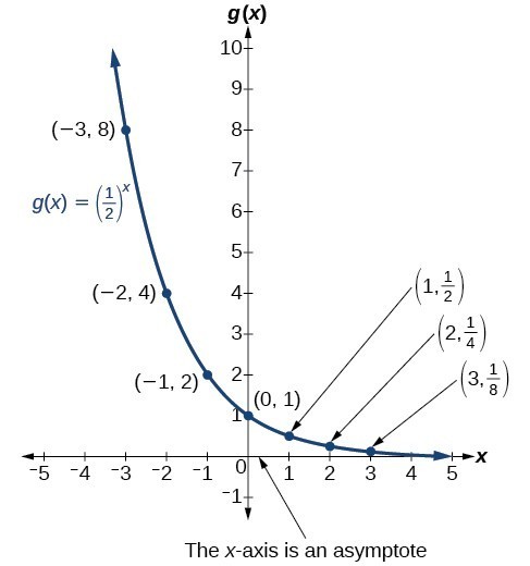
 The domain of [latex]g\left(x\right)={\left(\frac{1}{2}\right)}^{x}[/latex] is all real numbers; the range is [latex]\left(0,\infty \right)[/latex].

Characteristics of the Graph of  [latex]f(x) = b^{x}[/latex]

An exponential function of the form [latex]f\left(x\right)={b}^{x}[/latex], [latex]b>0[/latex], [latex]b\ne 1[/latex], has these characteristics:

• one-to-one function
• domain: [latex]\left(-\infty , \infty \right)[/latex]
• range: [latex]\left(0,\infty \right)[/latex]
• x-intercept: none
• y-intercept: [latex]\left(0,1\right)[/latex]
• increasing if [latex]b>1[/latex]
• decreasing if [latex]b<1[/latex]

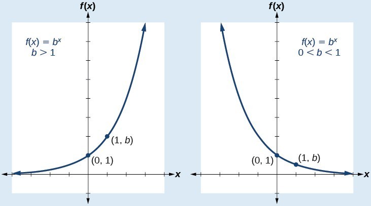
Compare the graphs of exponential growth and decay functions below.

In our first example, we will plot an exponential decay function where the base is between 0 and 1.

In the following video, we show another example of graphing an exponential function. The base of the exponential term is between [latex]0[/latex] and [latex]1[/latex], so this graph will represent decay.

In our next example, we will plot an exponential growth function where the base is greater than [latex]1[/latex].

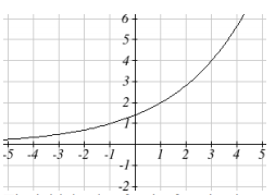
Example

Sketch a graph of [latex]f(x)={\sqrt{2}(\sqrt{2})}^{x}[/latex]. State the domain and range.

Show Solution

Before graphing, identify the behavior and create a table of points for the graph.

• Since b = [latex]\sqrt{2}[/latex], which is greater than one, we know the function is increasing, and we can verify this by creating a table of values. The left tail of the graph will get really close to the x-axis and the right tail will increase without bound.
• Create a table of points.
  

  x	[latex]–3[/latex]	[latex]–2[/latex]	[latex]–1[/latex]	[latex]0[/latex]	[latex]1[/latex]	[latex]2[/latex]	[latex]3[/latex]
  [latex]f\left(x\right)=\sqrt{2}{(\sqrt{2})}^{x}[/latex]	[latex]0.5[/latex]	[latex]0.71[/latex]	[latex]1[/latex]	[latex]1.41[/latex]	[latex]2[/latex]	[latex]2.83[/latex]	[latex]4[/latex]

• Plot the y-intercept, [latex]\left(0,1.41\right)[/latex], along with two other points. We can use [latex]\left(-1,1\right)[/latex] and [latex]\left(1,2\right)[/latex].

Draw a smooth curve connecting the points.

The domain is [latex]\left(-\infty ,\infty \right)[/latex]; the range is [latex]\left(0,\infty \right)[/latex].

Our next video example includes graphing an exponential growth function and defining the domain and range of the function.

Summary

Graphs of exponential growth functions will have a right tail that increases without bound and a left tail that gets really close to the x-axis. On the other hand, graphs of exponential decay functions will have a left tail that increases without bound and a right tail that gets really close to the x-axis. Points can be generated with a table of values which can then be used to graph the function.