Learning Outcomes
- Define direct variation and solve problems involving direct variation
- Define inverse variation and solve problems involving inverse variation
- Define joint variation and solve problems involving joint variation
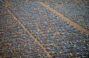
So many cars, so many tires.
Direct Variation
Variation equations are examples of rational formulas and are used to describe the relationship between variables. For example, imagine a parking lot filled with cars. The total number of tires in the parking lot is dependent on the total number of cars. Algebraically, you can represent this relationship with an equation.
[latex]\text{number of tires}=4\cdot\text{number of cars}[/latex]
The number [latex]4[/latex] tells you the rate at which cars and tires are related. You call the rate the constant of variation, also called the constant of proportionality. It’s a constant because this number does not change. Because the number of cars and the number of tires are linked by a constant, changes in the number of cars cause the number of tires to change in a proportional, steady way. This is an example of direct variation, where the number of tires varies directly with the number of cars.
You can use the car and tire equation as the basis for writing a general algebraic equation that will work for all examples of direct variation. In the example, the number of tires is the output, [latex]4[/latex] is the constant, and the number of cars is the input. Let’s enter those generic terms into the equation. You get [latex]y=kx[/latex]. That’s the formula for all direct variation equations.
[latex]\text{number of tires}=4\cdot\text{number of cars}\\\text{output}=\text{constant}\cdot\text{input}[/latex]
Example
Solve for k, the constant of variation, in a direct variation problem where [latex]y=300[/latex] and [latex]x=10[/latex].
In the video that follows, we present an example of solving a direct variation equation.
Try It
Inverse Variation
Another kind of variation is called inverse variation. In these equations, the output equals a constant divided by the input variable that is changing. In symbolic form, this is the equation [latex]y=\frac{k}{x}[/latex].
One example of an inverse variation is the speed required to travel between two cities in a given amount of time.
Let’s say you need to drive from Boston to Chicago, which is about [latex]1,000[/latex] miles. The more time you have, the slower you can go. If you want to get there in [latex]20[/latex] hours, you need to go [latex]50[/latex] miles per hour (assuming you don’t stop driving!), because [latex]\frac{1,000}{20}=50[/latex]. But if you can take [latex]40[/latex] hours to get there, you only have to average [latex]25[/latex] miles per hour, since [latex]\frac{1,000}{40}=25[/latex].
The equation for figuring out how fast to travel from the amount of time you have is [latex]speed=\frac{miles}{time}[/latex]. This equation should remind you of the distance formula [latex]d=rt[/latex]. If you solve [latex]d=rt[/latex] for r, you get [latex]r=\frac{d}{t}[/latex], or [latex]speed=\frac{miles}{time}[/latex].
In the case of the Boston to Chicago trip, you can write [latex]s=\frac{1,000}{t}[/latex]. Notice that this is the same form as the inverse variation function formula, [latex]y=\frac{k}{x}[/latex].
Example
Solve for k, the constant of variation, in an inverse variation problem where [latex]x=5[/latex] and [latex]y=25[/latex].
In the next example, we will find the water temperature in the ocean at a depth of [latex]500[/latex] meters. Water temperature is inversely proportional to depth in the ocean.
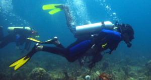
Water temperature in the ocean varies inversely with depth.
Example
The water temperature in the ocean varies inversely with the depth of the water. The deeper a person dives, the colder the water becomes. At a depth of [latex]1,000[/latex] meters, the water temperature is [latex]5º[/latex] Celsius. What is the water temperature at a depth of [latex]500[/latex] meters?
In the video that follows, we present an example of inverse variation.
Try It
Joint Variation
A third type of variation is called joint variation. Joint variation is the same as direct variation except there are two or more quantities. For example, the area of a rectangle can be found using the formula [latex]A=lw[/latex], where l is the length of the rectangle and w is the width of the rectangle. If you change the width of the rectangle, then the area changes and similarly if you change the length of the rectangle then the area will also change. You can say that the area of the rectangle “varies jointly with the length and the width of the rectangle.”
The formula for the volume of a cylinder, [latex]V=\pi {{r}^{2}}h[/latex] is another example of joint variation. The volume of the cylinder varies jointly with the square of the radius and the height of the cylinder. The constant of variation is [latex]\pi[/latex].
Example
The area of a triangle varies jointly with the lengths of its base and height. If the area of a triangle is [latex]30[/latex] inches[latex]^{2}[/latex] when the base is [latex]10[/latex] inches and the height is [latex]6[/latex] inches, find the variation constant and the area of a triangle whose base is [latex]15[/latex] inches and height is [latex]20[/latex] inches.
Finding k to be [latex]\frac{1}{2}[/latex] shouldn’t be surprising. You know that the area of a triangle is one-half base times height, [latex]A=\frac{1}{2}bh[/latex]. The [latex]\frac{1}{2}[/latex] in this formula is exactly the same [latex]\frac{1}{2}[/latex] that you calculated in this example!
In the following video, we show an example of finding the constant of variation for a jointly varying relation.
Try It
Direct, Joint, and Inverse Variation
k is the constant of variation. In all cases, [latex]k\neq0[/latex].
- Direct variation: [latex]y=kx[/latex]
- Inverse variation: [latex]y=\frac{k}{x}[/latex]
- Joint variation: [latex]y=kxz[/latex]
Summary
Rational formulas can be used to solve a variety of problems that involve rates, times, and work. Direct, inverse, and joint variation equations are examples of rational formulas. In direct variation, the variables have a direct relationship—as one quantity increases, the other quantity will also increase. As one quantity decreases, the other quantity decreases. In inverse variation, the variables have an inverse relationship—as one variable increases, the other variable decreases, and vice versa. Joint variation is the same as direct variation except there are two or more variables.
Candela Citations
- Screenshot: so many cars, so many tires. Provided by: Lumen Learning. License: CC BY: Attribution
- Screenshot: Water temperature in the ocean varies inversely with depth. Provided by: Lumen Learning. License: CC BY: Attribution
- Revision and Adaptation. Provided by: Lumen Learning. License: CC BY: Attribution
- Joint Variation: Determine the Variation Constant (Volume of a Cone). Authored by: James Sousa (Mathispower4u.com) for Lumen Learning. Located at: https://youtu.be/JREPATMScbM. License: CC BY: Attribution
- Unit 15: Rational Expressions, from Developmental Math: An Open Program. Provided by: Monterey Institute of Technology and Education. Located at: http://nrocnetwork.org/resources/downloads/nroc-math-open-textbook-units-1-12-pdf-and-word-formats/. License: CC BY: Attribution
- Ex: Direct Variation Application - Aluminum Can Usage. Authored by: James Sousa (Mathispower4u.com). Located at: https://youtu.be/DLPKiMD_ZZw. License: CC BY: Attribution
- Ex: Inverse Variation Application - Number of Workers and Job Time. Authored by: James Sousa (Mathispower4u.com) . Located at: https://youtu.be/y9wqI6Uo6_M. License: CC BY: Attribution