Aggregate Supply

The Aggregate Demand-Aggregate Supply model is designed to answer the questions of what determines the level of economic activity in the economy (i.e. what determines real GDP and employment), and what causes economic activity to speed up or slow down.

We can begin to answer these questions if we think about the concept of the aggregate production function, which we introduced in the context of economic growth. The aggregate production function shows the relationship between the resources (or factors of production) the economy has (e.g. labor, capital, technology, etc.) and the amount of output (i.e. real GDP) that can be produced. If all resources are fully employed, the resulting output is called Potential GDP. (Over time, as the economy obtains more resources as the labor force and capital stock grow and as technology improves, the economy produces more GDP. We have described this process as economic growth.)

Firms make decisions about what quantity of output to supply based on the profits they expect to earn. Profits, in turn, are also determined by the price of the outputs the firm sells and by the price of the inputs, like labor or raw materials, the firm needs to buy.

The previous paragraph included a critical assumption: full employment of resources. Why wouldn’t all resources be fully employed? Recall that when we discussed cyclical unemployment, we pointed out that wages are often sticky, that is, they don’t respond immediately to changes in demand for labor. The same thing may be true of other input prices. Let’s think about that in the context of an aggregate supply curve, showing the relationship between the aggregate price level and real GDP.

Aggregate supply (AS) refers to the total quantity of output (i.e. real GDP) firms will produce. The aggregate supply (AS) curve shows the total quantity of output firms will produce and sell (i.e, real GDP) at each aggregate price level, holding the price of inputs fixed.

Recall that the aggregate price level is an average of the prices of outputs in the economy. A decrease in the price level means that firms would like to reduce the wage rate they pay so they can maintain their profits. If wages are sticky downwards, labor becomes too expensive to keep fully employed, so firms layoff workers. (Economists would say that the real wage (W/P) is too high.) With fewer workers employed, firms produce less output and real GDP decreases. In short, when wages are sticky in response to changes in demand, then a lower aggregate price level corresponds to a lower level of real GDP. Similarly, an increase in the price level means that firms would like to raise wages, but it wages are sticky, labor becomes cheap so firms increase employment (or work hours) and real GDP increases.

Figure 1 shows an aggregate supply curve. In the following paragraphs, we will walk through the elements of the diagram one at a time: the horizontal and vertical axes, the aggregate supply curve itself, and the meaning of the potential GDP vertical line.

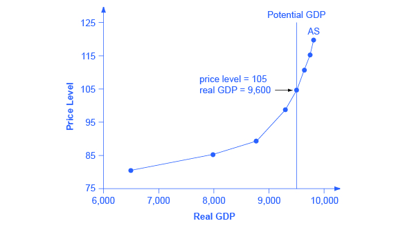
Figure 1. The Aggregate Supply Curve. Aggregate supply (AS) slopes up, because as the price level for outputs rises, with the price of inputs remaining fixed, firms have an incentive to produce more and to earn higher profits. The potential GDP line shows the maximum that the economy can produce with full employment of workers and physical capital.

The horizontal axis of the diagram shows real GDP—that is, the level of GDP adjusted for inflation. The vertical axis shows the aggregate price level.  As the price level rises, the aggregate quantity of goods and services produced rises as well. Why? The price level shown on the vertical axis represents the average price for final goods or outputs purchased in the economy, i.e. the GDP deflator.  It is not the price level for intermediate goods and services that are inputs to production.  Thus, the AS curve describes how suppliers will react to a higher price level for outputs of goods and services, while holding the prices of inputs like labor and energy constant. If firms across the economy face a situation where the price level of what they produce and sell is rising, but their costs of production are not rising, then the lure of higher profits will induce them to expand production.

The slope of an AS curve changes from nearly flat at its far left to nearly vertical at its far right. At the far left of the aggregate supply curve, the level of output in the economy is far below potential GDP, which is defined as the quantity that an economy can produce by fully employing its resources of labor, physical capital, and technology, in the context of its existing market and legal institutions. At these relatively low levels of output, levels of unemployment are high, and many factories are running only part-time, or have closed their doors. In this situation, a relatively small increase in the prices of the outputs that businesses sell—while making the assumption of no rise in input prices—can encourage a considerable surge in real GDP because so many workers and factories are ready to swing into production.

As the quantity produced increases, however, certain firms and industries will start running into limits: perhaps nearly all of the expert workers in a certain industry will have jobs or factories in certain geographic areas or industries will be running at full speed. In the intermediate area of the AS curve, a higher price level for outputs continues to encourage a greater quantity of output—but as the increasingly steep upward slope of the aggregate supply curve shows, the increase in GDP in response to a given rise in the price level will not be quite as large.

At the far right, the aggregate supply curve becomes nearly vertical. At this quantity, higher prices for outputs cannot encourage additional output, because even if firms want to expand output, the inputs of labor and machinery in the economy are fully employed. In this example, the vertical line in the exhibit shows that potential GDP occurs at a total output of 9,500. When an economy is operating at its potential GDP, machines and factories are running at capacity, and the unemployment rate is relatively low—at the natural rate of unemployment. For this reason, potential GDP is sometimes also called full-employment GDP.

Defining SRAS and LRAS

If we define the short run as the period of time that wages are sticky, then we can describe the positive relationship between P & Q as the short run aggregate supply (SRAS) curve, shown above in Figure 1 as AS.

In the long run, however, all wages and prices are fully flexible. As a consequence, all resources will be fully employed and real GDP will equal potential, regardless of the price level. Thus, in the long run, real GDP will be independent of the price level, and the long run aggregate supply (LRAS) curve will be a vertical line at potential (or the full employment level of) GDP. This can be seen on a graph as potential GDP (as in Figure 1) or as LRAS.

The Aggregate Demand Curve

Aggregate demand (AD) refers to total spending in an economy on domestic goods and services. (Strictly speaking, AD is what economists call total planned expenditure. You’ll learn about this in more detail in the Keynesian module.) It includes all four components of spending: consumption expenditure, investment expenditure, government expenditure, and net export expenditure (exports minus imports). This demand is determined by a number of factors, but one of them is the aggregate price level. The aggregate demand (AD) curve shows the total spending on domestic goods and services at each price level.

Figure 2 presents an aggregate demand (AD) curve. Just like the aggregate supply curve, the horizontal axis shows real GDP and the vertical axis shows the price level. The AD curve is downward sloping from left to right, which means that a decrease in the aggregate price level leads to an increase in the amount of total spending on domestic goods and services. Even though the AD curve looks like a microeconomic demand curve, it doesn’t operate the same way. Rather, the reasons behind this negative relationship are related to how changes in the price level affect the different components of aggregate demand. Recall that aggregate demand consists of consumption spending (C), investment spending (I), government spending (G), and spending on exports (X) minus imports (M): C + I + G + X – M.

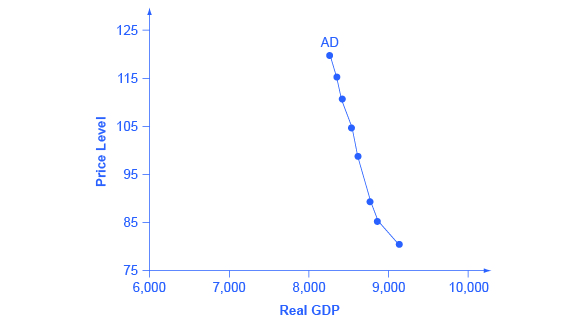
Figure 2. The Aggregate Demand Curve. Aggregate demand (AD) slopes down, showing that, as the price level rises, the amount of total spending on domestic goods and services declines.

There are three specific reasons for why AD curves are downward sloping. These are the wealth effect, the interest rate effect and the foreign price effect. Each of them tends to affect a different component of aggregate demand.

The wealth effect holds that as the price level increases, the buying power of savings that people have stored up in bank accounts and other assets will diminish, eaten away to some extent by inflation. Because a rise in the price level reduces people’s wealth, consumption spending will fall as the price level rises.

The interest rate effect is that as prices for outputs rise, the same purchases will take more money or credit to accomplish. This additional demand for money and credit will push interest rates higher. In turn, higher interest rates will reduce borrowing by businesses for investment purposes and reduce borrowing by households for homes and cars—thus reducing consumption and investment spending.

The foreign price effect points out that if prices rise in the United States while remaining fixed in other countries, then goods in the United States will be relatively more expensive compared to goods in the rest of the world. U.S. exports will be relatively more expensive, and the quantity of exports sold will fall. U.S. imports from abroad will be relatively cheaper, so the quantity of imports will rise. Thus, a higher domestic price level, relative to price levels in other countries, will reduce net export expenditures.

Truth be told, among economists all three of these effects are controversial, in part because they do not seem to be very large. For this reason, the aggregate demand curve in Figure 2 slopes downward fairly steeply; the steep slope indicates that a higher price level for final outputs reduces aggregate demand for all three of these reasons, but that the change in the quantity of aggregate demand as a result of changes in price level is not very large.

Try It

Glossary

aggregate demand (AD):

the amount of total spending on domestic goods and services in an economy

aggregate supply (AS):

the total quantity of output (i.e. real GDP) firms will produce and sell

aggregate demand (AD) curve:

the total spending on domestic goods and services at each aggregate price level

aggregate supply (AS) curve:

the total quantity of output (i.e. real GDP) that firms will produce and sell at each aggregate price level

aggregate demand/aggregate supply model:

a model that shows the equilibrium real GDP & aggregate price level for the macro economy, based on the interaction between aggregate demand and aggregate supply

foreign price effect:

if prices rise in the United States while remaining fixed in other countries, then goods in the United States will be relatively more expensive compared to goods in the rest of the world

interest rate effect:

as the aggregate price level rises, the same purchases will take more money or credit to accomplish, driving up interest rates

long run:

period of time during which all wages and prices are fully flexible

long run aggregate supply (LRAS) curve:

vertical line at potential GDP showing no relationship between the aggregate price level and real GDP in the long run

potential GDP:

the maximum quantity that an economy can produce given full employment of its existing levels of labor, physical capital, technology, and institutions; also known as full employment GDP

short run:

period of time during which wages (and some prices) are sticky in response to a change in demand

short run aggregate supply (SRAS) curve:

positive short run relationship between the aggregate price level and real GDP, holding the prices of inputs fixed

wealth effect:

as price level increases, the buying power of savings that people have stored up in bank accounts and other assets will diminish