Credibility makes our messages believable, and a believable message is more likely to be remembered than one that is not. But gaining credibility is not so easy. As Chip and Dan Heath note in Made to Stick: “If we’re trying to persuade a skeptical audience to believe a new message, the reality is that we’re fighting an uphill battle against a lifetime of personal learning and social relationships.”^[1]

In 2019, Americans spent almost half a billion dollars on Halloween costumes for their pets.

So how can we add credibility to our words? One way is to use statistics. Statistics can offer credibility by grounding a claim in verifiable numbers. If I say, “Americans spend a lot on their pets,” that’s a judgment on my part—I could equally say, “Americans spend too much on their pets” or “Americans spend too little on their pets.” Now imagine if I say, “According to the American Pet Products Association, Americans spent over $72 billion on their pets in 2018.” Here we are not dealing with my judgment (how much is a lot?), but rather with a verifiable figure. An audience member could look up the source and even track down how the APPA arrived at this number.^[2]

We should not assume, however, that this statistic alone makes our argument. Statistics only have meaning in context. For instance, I could relativize this number (and perhaps minimize it) by pointing out that Americans also spend nearly that much on soft drinks each year ($65 billion)^[3], or take it up a notch by pointing out that in 2019, Americans spent almost half a billion dollars on Halloween costumes for their pets.^[4]

In order to use statistics effectively and responsibly, it’s important to review some key concepts.

Probability

One of the simplest illustrations of probability is a coin flip. For each flip, there is a 50% probability of heads and a 50% probability of tails.

Probability is a mathematical tool used to study randomness. It deals with the chance of an event occurring. For example, if you toss a fair coin four times, the outcomes may not be two heads and two tails. However, if you toss the same coin 4,000 times, the outcomes will be close to half heads and half tails. The expected theoretical probability of heads in any one toss is 1/2 or 0.5. Even though the outcomes of a few repetitions are uncertain, there is a regular pattern of outcomes when there are many repetitions. The English statistician Karl Pearson once tossed a coin 24,000 times with a result of 12,012 heads.^[5]

The theory of probability began with the study of games of chance such as poker. Predictions take the form of probabilities. To predict the likelihood of an earthquake, rain, or whether you will get an A in this course, we use probabilities. Doctors use probability to determine the chance of a vaccine causing the disease the vaccination is supposed to prevent. A stockbroker uses probability to determine the rate of return on a client’s investments.

P-Value

If a process is subject to probability and chance, it becomes difficult to determine whether a given effect is due to the input being tested or just random chance. In statistics, a p–value is a measure of the probability that an effect could be explained by random chance, and has nothing to do with the variables being tested. The p-value is related to the concept of statistical significance. If a p-value is high—that is, if there’s a fairly high probability that the effect is due to chance—then the result of the test is not considered statistically significant. Both of these concepts contain a lot of theory and math, but they’re important to be aware of, since the question of statistical significance is one of the main critical questions we should ask of any statistical argument.

Population and Sample

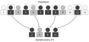
Ideally, a population is sampled systematically. In this simple system, every third person is included in the sample.

In statistics, we generally want to study a population. You can think of a population as a collection of persons, things, or objects under study. To study the population, we select a sample. The idea of sampling is to select a portion (or subset) of the larger population and study that portion (the sample) to gain information about the population. Data is the result of sampling from a population.

Because it takes a lot of time and money to examine an entire population, sampling is a very practical technique. If you wished to compute the overall grade point average at your school, it would make sense to select a sample of students who attend the school. The data collected from the sample would be the students’ grade point averages. In presidential elections, opinion poll samples of [latex]1,000[/latex]–[latex]2,000[/latex] people are taken. The opinion poll is supposed to represent the views of the people in the entire country. Manufacturers of canned carbonated drinks take samples to determine if a [latex]16[/latex] ounce can contains [latex]16[/latex] ounces of carbonated drink.

Generalizability

One of the main concerns in the field of statistics is how accurately a particular statistic estimates a given property of the population. The accuracy really depends on how well the sample represents the population. The sample must contain the characteristics of the population in order to be a representative sample. The margin of error is a statistic expressing the amount of random sampling error in the results of a survey. The larger the margin of error, the less confidence one should have that a poll result would reflect the result of a survey of the entire population.

Variables

A variable, notated by capital letters such as [latex]X[/latex] and [latex]Y[/latex], is a characteristic of interest for each person or thing in a population. Variables may be numerical or categorical. Numerical variables take on values with equal units such as weight in pounds and time in hours. Categorical variables place the person or thing into a category. If we let [latex]X[/latex] equal the number of points earned by one math student at the end of a term, then [latex]X[/latex] is a numerical variable. If we let [latex]Y[/latex] be a person’s party affiliation, then some examples of [latex]Y[/latex] include Republican, Democrat, and Independent. [latex]Y[/latex] is a categorical variable. We could do some math with values of [latex]X[/latex] (calculate the average number of points earned, for example), but it makes no sense to do math with values of [latex]Y[/latex] (calculating an average party affiliation makes no sense).

Data are the actual values of the variable. They may be numbers or they may be words. Datum is a single value. When you have data for a set of variables, the patterns of variation in the data are called the distribution of the variable.

Mean, Median, and Proportion

When working with a set of data, mean, median, and proportion are important concepts. If you were to take three exams in your math classes and obtain scores of [latex]86[/latex], [latex]75[/latex], and [latex]92[/latex], you would calculate your mean score by adding the three exam scores and dividing by three (your mean score would be [latex]84.3[/latex] to one decimal place). With some data sets, the mean fails to capture a reasonable relationship between the values. If your math class were taught by billionaire Jeff Bezos, the mean net worth of everyone in the room will be something like 58 billion dollars. In cases like this, we might want to use the median, which means the middle term in a series ordered by magnitude. Imagine, in that same math class, if one test is particularly hard, and you and your classmates get grades of 30%, 12%, 23%, 22%, and 100% (hopefully that one’s you!). While the mean score would be 37.4%, the median would be 23% (remember to order those numbers to get the median!: 12%, 22%, 23%, 30%, 100%). Which would you use to petition the instructor to throw out that test? If, in your math class, there are [latex]40[/latex] students and [latex]22[/latex] are in-state and [latex]18[/latex] are out-of-state, then the proportion of in-state students is [latex]\displaystyle\frac{{22}}{{40}}[/latex] and the proportion of out-of-state students is [latex]\displaystyle\frac{{18}}{{40}}[/latex].

NOTE: The words mean and average are often used interchangeably. The substitution of one word for the other is common practice. The technical term is arithmetic mean, and average is technically a center location. However, in practice among non-statisticians, average is commonly accepted for arithmetic mean.