Learning Outcomes
- Compute a conditional probability for an event
- Use Baye’s theorem to compute a conditional probability
- Calculate the expected value of an event
In the next section, we will explore more complex conditional probabilities and ways to compute them. Conditional probabilities can give us information such as the likelihood of getting a positive test result for a disease without actually having the disease. If a doctor thinks the chances that a positive test result nearly guarantees that a patient has a disease, they might begin an unnecessary and possibly harmful treatment regimen on a healthy patient. If you were to get a positive test result, knowing the likelihood of getting a false positive can guide you to get a second opinion.
Bayes’ Theorem
In this section we concentrate on the more complex conditional probability problems we began looking at in the last section.

For example, suppose a certain disease has an incidence rate of 0.1% (that is, it afflicts 0.1% of the population). A test has been devised to detect this disease. The test does not produce false negatives (that is, anyone who has the disease will test positive for it), but the false positive rate is 5% (that is, about 5% of people who take the test will test positive, even though they do not have the disease). Suppose a randomly selected person takes the test and tests positive. What is the probability that this person actually has the disease?
There are two ways to approach the solution to this problem. One involves an important result in probability theory called Bayes’ theorem. We will discuss this theorem a bit later, but for now we will use an alternative and, we hope, much more intuitive approach.
Let’s break down the information in the problem piece by piece as an example.
example
Suppose a certain disease has an incidence rate of 0.1% (that is, it afflicts 0.1% of the population). The percentage 0.1% can be converted to a decimal number by moving the decimal place two places to the left, to get 0.001. In turn, 0.001 can be rewritten as a fraction: 1/1000. This tells us that about 1 in every 1000 people has the disease. (If we wanted we could write P(disease)=0.001.)
A test has been devised to detect this disease. The test does not produce false negatives (that is, anyone who has the disease will test positive for it). This part is fairly straightforward: everyone who has the disease will test positive, or alternatively everyone who tests negative does not have the disease. (We could also say P(positive | disease)=1.)
The false positive rate is 5% (that is, about 5% of people who take the test will test positive, even though they do not have the disease). This is even more straightforward. Another way of looking at it is that of every 100 people who are tested and do not have the disease, 5 will test positive even though they do not have the disease. (We could also say that P(positive | no disease)=0.05.)
Suppose a randomly selected person takes the test and tests positive. What is the probability that this person actually has the disease? Here we want to compute P(disease|positive). We already know that P(positive|disease)=1, but remember that conditional probabilities are not equal if the conditions are switched.
Rather than thinking in terms of all these probabilities we have developed, let’s create a hypothetical situation and apply the facts as set out above. First, suppose we randomly select 1000 people and administer the test. How many do we expect to have the disease? Since about 1/1000 of all people are afflicted with the disease, 1/1000 of 1000 people is 1. (Now you know why we chose 1000.) Only 1 of 1000 test subjects actually has the disease; the other 999 do not.
We also know that 5% of all people who do not have the disease will test positive. There are 999 disease-free people, so we would expect (0.05)(999)=49.95 (so, about 50) people to test positive who do not have the disease.
Now back to the original question, computing P(disease|positive). There are 51 people who test positive in our example (the one unfortunate person who actually has the disease, plus the 50 people who tested positive but don’t). Only one of these people has the disease, so
P(disease | positive) [latex]\approx\frac{1}{51}\approx0.0196[/latex]
or less than 2%. Does this surprise you? This means that of all people who test positive, over 98% do not have the disease.
The answer we got was slightly approximate, since we rounded 49.95 to 50. We could redo the problem with 100,000 test subjects, 100 of whom would have the disease and (0.05)(99,900)=4995 test positive but do not have the disease, so the exact probability of having the disease if you test positive is
P(disease | positive) [latex]\approx\frac{100}{5095}\approx0.0196[/latex]
which is pretty much the same answer.
But back to the surprising result. Of all people who test positive, over 98% do not have the disease. If your guess for the probability a person who tests positive has the disease was wildly different from the right answer (2%), don’t feel bad. The exact same problem was posed to doctors and medical students at the Harvard Medical School 25 years ago and the results revealed in a 1978 New England Journal of Medicine article. Only about 18% of the participants got the right answer. Most of the rest thought the answer was closer to 95% (perhaps they were misled by the false positive rate of 5%).
So at least you should feel a little better that a bunch of doctors didn’t get the right answer either (assuming you thought the answer was much higher). But the significance of this finding and similar results from other studies in the intervening years lies not in making math students feel better but in the possibly catastrophic consequences it might have for patient care. If a doctor thinks the chances that a positive test result nearly guarantees that a patient has a disease, they might begin an unnecessary and possibly harmful treatment regimen on a healthy patient. Or worse, as in the early days of the AIDS crisis when being HIV-positive was often equated with a death sentence, the patient might take a drastic action and commit suicide.
This example is worked through in detail in the video here.
As we have seen in this hypothetical example, the most responsible course of action for treating a patient who tests positive would be to counsel the patient that they most likely do not have the disease and to order further, more reliable, tests to verify the diagnosis.
One of the reasons that the doctors and medical students in the study did so poorly is that such problems, when presented in the types of statistics courses that medical students often take, are solved by use of Bayes’ theorem, which is stated as follows:
Bayes’ Theorem
[latex]P(A|B)=\frac{P(A)P(B|A)}{P(A)P(B|A)+P(\bar{A})P(B|\bar{A})}[/latex]
In our earlier example, this translates to
[latex]P(\text{disease}|\text{positive})=\frac{P(\text{disease})P(\text{positive}|\text{disease})}{P(\text{disease})P(\text{positive}|\text{disease})+P(\text{nodisease})P(\text{positive}|\text{nodisease})}[/latex]
Plugging in the numbers gives
[latex]P(\text{disease}|\text{positive})=\frac{(0.001)(1)}{(0.001)(1)+(0.999)(0.05)}\approx0.0196[/latex]
which is exactly the same answer as our original solution.
The problem is that you (or the typical medical student, or even the typical math professor) are much more likely to be able to remember the original solution than to remember Bayes’ theorem. Psychologists, such as Gerd Gigerenzer, author of Calculated Risks: How to Know When Numbers Deceive You, have advocated that the method involved in the original solution (which Gigerenzer calls the method of “natural frequencies”) be employed in place of Bayes’ Theorem. Gigerenzer performed a study and found that those educated in the natural frequency method were able to recall it far longer than those who were taught Bayes’ theorem. When one considers the possible life-and-death consequences associated with such calculations it seems wise to heed his advice.
example
A certain disease has an incidence rate of 2%. If the false negative rate is 10% and the false positive rate is 1%, compute the probability that a person who tests positive actually has the disease.
View the following for more about this example.
Try It
Counting
Counting? You already know how to count or you wouldn’t be taking a college-level math class, right? Well yes, but what we’ll really be investigating here are ways of counting efficiently. When we get to the probability situations a bit later in this chapter we will need to count some very large numbers, like the number of possible winning lottery tickets. One way to do this would be to write down every possible set of numbers that might show up on a lottery ticket, but believe me: you don’t want to do this.
Basic Counting
We will start, however, with some more reasonable sorts of counting problems in order to develop the ideas that we will soon need.
example
Suppose at a particular restaurant you have three choices for an appetizer (soup, salad or breadsticks) and five choices for a main course (hamburger, sandwich, quiche, fajita or pizza). If you are allowed to choose exactly one item from each category for your meal, how many different meal options do you have?
Solution 1: One way to solve this problem would be to systematically list each possible meal:
soup + hamburger soup + sandwich soup + quiche
soup + fajita soup + pizza salad + hamburger
salad + sandwich salad + quiche salad + fajita
salad + pizza breadsticks + hamburger breadsticks + sandwich
breadsticks + quiche breadsticks + fajita breadsticks + pizza
Assuming that we did this systematically and that we neither missed any possibilities nor listed any possibility more than once, the answer would be 15. Thus you could go to the restaurant 15 nights in a row and have a different meal each night.
Solution 2: Another way to solve this problem would be to list all the possibilities in a table:
| hamburger | sandwich | quiche | fajita | pizza | |
| soup | soup+burger | ||||
| salad | salad+burger | ||||
| bread | etc |
In each of the cells in the table we could list the corresponding meal: soup + hamburger in the upper left corner, salad + hamburger below it, etc. But if we didn’t really care what the possible meals are, only how many possible meals there are, we could just count the number of cells and arrive at an answer of 15, which matches our answer from the first solution. (It’s always good when you solve a problem two different ways and get the same answer!)
Solution 3: We already have two perfectly good solutions. Why do we need a third? The first method was not very systematic, and we might easily have made an omission. The second method was better, but suppose that in addition to the appetizer and the main course we further complicated the problem by adding desserts to the menu: we’ve used the rows of the table for the appetizers and the columns for the main courses—where will the desserts go? We would need a third dimension, and since drawing 3-D tables on a 2-D page or computer screen isn’t terribly easy, we need a better way in case we have three categories to choose form instead of just two.
So, back to the problem in the example. What else can we do? Let’s draw a tree diagram:
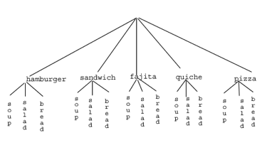
This is called a “tree” diagram because at each stage we branch out, like the branches on a tree. In this case, we first drew five branches (one for each main course) and then for each of those branches we drew three more branches (one for each appetizer). We count the number of branches at the final level and get (surprise, surprise!) 15.
If we wanted, we could instead draw three branches at the first stage for the three appetizers and then five branches (one for each main course) branching out of each of those three branches.
OK, so now we know how to count possibilities using tables and tree diagrams. These methods will continue to be useful in certain cases, but imagine a game where you have two decks of cards (with 52 cards in each deck) and you select one card from each deck. Would you really want to draw a table or tree diagram to determine the number of outcomes of this game?
Let’s go back to the previous example that involved selecting a meal from three appetizers and five main courses, and look at the second solution that used a table. Notice that one way to count the number of possible meals is simply to number each of the appropriate cells in the table, as we have done above. But another way to count the number of cells in the table would be multiply the number of rows (3) by the number of columns (5) to get 15. Notice that we could have arrived at the same result without making a table at all by simply multiplying the number of choices for the appetizer (3) by the number of choices for the main course (5). We generalize this technique as the basic counting rule:
Basic Counting Rule
If we are asked to choose one item from each of two separate categories where there are m items in the first category and n items in the second category, then the total number of available choices is m · n.
This is sometimes called the multiplication rule for probabilities.
example
There are 21 novels and 18 volumes of poetry on a reading list for a college English course. How many different ways can a student select one novel and one volume of poetry to read during the quarter?
The Basic Counting Rule can be extended when there are more than two categories by applying it repeatedly, as we see in the next example.
example
Suppose at a particular restaurant you have three choices for an appetizer (soup, salad or breadsticks), five choices for a main course (hamburger, sandwich, quiche, fajita or pasta) and two choices for dessert (pie or ice cream). If you are allowed to choose exactly one item from each category for your meal, how many different meal options do you have?
Try It
Example
A quiz consists of 3 true-or-false questions. In how many ways can a student answer the quiz?
Basic counting examples from this section are described in the following video.
Permutations
In this section we will develop an even faster way to solve some of the problems we have already learned to solve by other means. Let’s start with a couple examples.
example
How many different ways can the letters of the word MATH be rearranged to form a four-letter code word?
In this example, we needed to calculate n · (n – 1) · (n – 2) ··· 3 · 2 · 1. This calculation shows up often in mathematics, and is called the factorial, and is notated n!
Factorial
n! = n · (n – 1) · (n – 2) ··· 3 · 2 · 1
Try It
example
How many ways can five different door prizes be distributed among five people?
Try It
Now we will consider some slightly different examples.
examples
A charity benefit is attended by 25 people and three gift certificates are given away as door prizes: one gift certificate is in the amount of $100, the second is worth $25 and the third is worth $10. Assuming that no person receives more than one prize, how many different ways can the three gift certificates be awarded?
Example
Eight sprinters have made it to the Olympic finals in the 100-meter race. In how many different ways can the gold, silver and bronze medals be awarded?
Factorial examples are worked in this video.
We can generalize the situation in the two examples above to any problem without replacement where the order of selection is important. If we are arranging in order r items out of n possibilities (instead of 3 out of 25 or 3 out of 8 as in the previous examples), the number of possible arrangements will be given by
n · (n – 1) · (n – 2) ··· (n – r + 1)
If you don’t see why (n — r + 1) is the right number to use for the last factor, just think back to the first example in this section, where we calculated 25 · 24 · 23 to get 13,800. In this case n = 25 and r = 3, so n — r + 1 = 25 — 3 + 1 = 23, which is exactly the right number for the final factor.
Now, why would we want to use this complicated formula when it’s actually easier to use the Basic Counting Rule, as we did in the first two examples? Well, we won’t actually use this formula all that often; we only developed it so that we could attach a special notation and a special definition to this situation where we are choosing r items out of n possibilities without replacement and where the order of selection is important. In this situation we write:
Permutations
nPr = n · (n – 1) · (n – 2) ··· (n – r + 1)
We say that there are nPr permutations of size r that may be selected from among n choices without replacement when order matters.
It turns out that we can express this result more simply using factorials.
[latex]{}_{n}{{P}_{r}}=\frac{n!}{(n-r)!}[/latex]
In practicality, we usually use technology rather than factorials or repeated multiplication to compute permutations.
example
I have nine paintings and have room to display only four of them at a time on my wall. How many different ways could I do this?
Example
How many ways can a four-person executive committee (president, vice-president, secretary, treasurer) be selected from a 16-member board of directors of a non-profit organization?
View this video to see more about the permutations examples.
Try It
How many 5 character passwords can be made using the letters A through Z
- if repeats are allowed
- if no repeats are allowed
Combinations
In the previous section we considered the situation where we chose r items out of n possibilities without replacement and where the order of selection was important. We now consider a similar situation in which the order of selection is not important.
Example
A charity benefit is attended by 25 people at which three $50 gift certificates are given away as door prizes. Assuming no person receives more than one prize, how many different ways can the gift certificates be awarded?
We can generalize the situation in this example above to any problem of choosing a collection of items without replacement where the order of selection is not important. If we are choosing r items out of n possibilities (instead of 3 out of 25 as in the previous examples), the number of possible choices will be given by [latex]\frac{{}_{n}{{P}_{r}}}{{}_{r}{{P}_{r}}}[/latex], and we could use this formula for computation. However this situation arises so frequently that we attach a special notation and a special definition to this situation where we are choosing r items out of n possibilities without replacement where the order of selection is not important.
Combinations
[latex]{}_{n}{{C}_{r}}=\frac{{}_{n}{{P}_{r}}}{{}_{r}{{P}_{r}}}[/latex]
We say that there are nCr combinations of size r that may be selected from among n choices without replacement where order doesn’t matter.
We can also write the combinations formula in terms of factorials:
[latex]{}_{n}{{C}_{r}}=\frac{n!}{(n-r)!r!}[/latex]
Example
A group of four students is to be chosen from a 35-member class to represent the class on the student council. How many ways can this be done?
View the following for more explanation of the combinations examples.
Try It
The United States Senate Appropriations Committee consists of 29 members; the Defense Subcommittee of the Appropriations Committee consists of 19 members. Disregarding party affiliation or any special seats on the Subcommittee, how many different 19-member subcommittees may be chosen from among the 29 Senators on the Appropriations Committee?
In the preceding Try It problem we assumed that the 19 members of the Defense Subcommittee were chosen without regard to party affiliation. In reality this would never happen: if Republicans are in the majority they would never let a majority of Democrats sit on (and thus control) any subcommittee. (The same of course would be true if the Democrats were in control.) So let’s consider the problem again, in a slightly more complicated form:
Example
The United States Senate Appropriations Committee consists of 29 members, 15 Republicans and 14 Democrats. The Defense Subcommittee consists of 19 members, 10 Republicans and 9 Democrats. How many different ways can the members of the Defense Subcommittee be chosen from among the 29 Senators on the Appropriations Committee?
This example is worked through below.
Probability Using Permutations and Combinations
We can use permutations and combinations to help us answer more complex probability questions.
examples
A 4 digit PIN number is selected. What is the probability that there are no repeated digits?
Try It
Example
In a certain state’s lottery, 48 balls numbered 1 through 48 are placed in a machine and six of them are drawn at random. If the six numbers drawn match the numbers that a player had chosen, the player wins $1,000,000. In this lottery, the order the numbers are drawn in doesn’t matter. Compute the probability that you win the million-dollar prize if you purchase a single lottery ticket.
Example
In the state lottery from the previous example, if five of the six numbers drawn match the numbers that a player has chosen, the player wins a second prize of $1,000. Compute the probability that you win the second prize if you purchase a single lottery ticket.
The previous examples are worked in the following video.
examples
Compute the probability of randomly drawing five cards from a deck and getting exactly one Ace.
Example
Compute the probability of randomly drawing five cards from a deck and getting exactly two Aces.
View the following for further demonstration of these examples.
Try It
Birthday Problem
Let’s take a pause to consider a famous problem in probability theory:
Take a guess at the answer to the above problem. Was your guess fairly low, like around 10%? That seems to be the intuitive answer (30/365, perhaps?). Let’s see if we should listen to our intuition. Let’s start with a simpler problem, however.
example
Suppose three people are in a room. What is the probability that there is at least one shared birthday among these three people?
Suppose five people are in a room. What is the probability that there is at least one shared birthday among these five people?
Suppose 30 people are in a room. What is the probability that there is at least one shared birthday among these 30 people?
The birthday problem is examined in detail in the following.
If you like to bet, and if you can convince 30 people to reveal their birthdays, you might be able to win some money by betting a friend that there will be at least two people with the same birthday in the room anytime you are in a room of 30 or more people. (Of course, you would need to make sure your friend hasn’t studied probability!) You wouldn’t be guaranteed to win, but you should win more than half the time.
This is one of many results in probability theory that is counterintuitive; that is, it goes against our gut instincts.
Try It
Suppose 10 people are in a room. What is the probability that there is at least one shared birthday among these 10 people?
Expected Value
Repeating Procedures Over Time
Expected value is perhaps the most useful probability concept we will discuss. It has many applications, from insurance policies to making financial decisions, and it’s one thing that the casinos and government agencies that run gambling operations and lotteries hope most people never learn about.
example
In the casino game roulette, a wheel with 38 spaces (18 red, 18 black, and 2 green) is spun. In one possible bet, the player bets $1 on a single number. If that number is spun on the wheel, then they receive $36 (their original $1 + $35). Otherwise, they lose their $1. On average, how much money should a player expect to win or lose if they play this game repeatedly?
Expected Value
- Expected Value is the average gain or loss of an event if the procedure is repeated many times.
We can compute the expected value by multiplying each outcome by the probability of that outcome, then adding up the products.
Try It
You purchase a raffle ticket to help out a charity. The raffle ticket costs $5. The charity is selling 2000 tickets. One of them will be drawn and the person holding the ticket will be given a prize worth $4000. Compute the expected value for this raffle.
Example
In a certain state’s lottery, 48 balls numbered 1 through 48 are placed in a machine and six of them are drawn at random. If the six numbers drawn match the numbers that a player had chosen, the player wins $1,000,000. If they match 5 numbers, then win $1,000. It costs $1 to buy a ticket. Find the expected value.
View more about the expected value examples in the following video.
Try It
In general, if the expected value of a game is negative, it is not a good idea to play the game, since on average you will lose money. It would be better to play a game with a positive expected value (good luck trying to find one!), although keep in mind that even if the average winnings are positive it could be the case that most people lose money and one very fortunate individual wins a great deal of money. If the expected value of a game is 0, we call it a fair game, since neither side has an advantage.
Try It
A friend offers to play a game, in which you roll 3 standard 6-sided dice. If all the dice roll different values, you give him $1. If any two dice match values, you get $2. What is the expected value of this game? Would you play?
Expected value also has applications outside of gambling. Expected value is very common in making insurance decisions.
Example
A 40-year-old man in the U.S. has a 0.242% risk of dying during the next year.[1] An insurance company charges $275 for a life-insurance policy that pays a $100,000 death benefit. What is the expected value for the person buying the insurance?
The insurance applications of expected value are detailed in the following video.
Not surprisingly, the expected value is negative; the insurance company can only afford to offer policies if they, on average, make money on each policy. They can afford to pay out the occasional benefit because they offer enough policies that those benefit payouts are balanced by the rest of the insured people.
For people buying the insurance, there is a negative expected value, but there is a security that comes from insurance that is worth that cost.
Candela Citations
- Introduction and Learning Outcomes. Provided by: Lumen Learning. License: CC BY: Attribution
- Revision and Adaptation. Provided by: Lumen Learning. License: CC BY: Attribution
- Math in Society. Authored by: David Lippman. Located at: http://www.opentextbookstore.com/mathinsociety/. License: CC BY-SA: Attribution-ShareAlike
- Bayes' Theorem MMB 01. Authored by: mattbuck. Located at: https://commons.wikimedia.org/wiki/File:Bayes%27_Theorem_MMB_01.jpg. License: CC BY-SA: Attribution-ShareAlike
- Probability of a diesase given a positive test: Bayes Theorem ex1. Authored by: OCLPhase2's channel. Located at: https://youtu.be/hXevfqsBino. License: CC BY: Attribution
- Probability of a disease given a positive test: Bayes Theorem ex2. Authored by: OCLPhase2's channel. Located at: https://youtu.be/_c3xZvHto3k. License: CC BY: Attribution
- Basic counting. Authored by: OCLPhase2's channel. Located at: https://youtu.be/fROqcu-ekkw. License: CC BY: Attribution
- Counting using the factorial. Authored by: OCLPhase2's channel. Located at: https://youtu.be/9maoGi5fd_M. License: CC BY: Attribution
- Permutations. Authored by: OCLPhase2's channel. Located at: https://youtu.be/xlyX2UJMJQI. License: CC BY: Attribution
- Combinations. Authored by: OCLPhase2's channel. Located at: https://youtu.be/W8kd4YosbzE. License: CC BY: Attribution
- Combinations 2. Authored by: OCLPhase2's channel. Located at: https://youtu.be/Xqc2sdYN7xo. License: CC BY: Attribution
- Probabilities using combinations. Authored by: OCLPhase2's channel. Located at: https://youtu.be/b9LFbB_aNAo. License: CC BY: Attribution
- Probabilities using combinations: cards. Authored by: OCLPhase2's channel. Located at: https://youtu.be/RU3e3KTkjoA. License: CC BY: Attribution
- Probability: the birthday problem. Authored by: OCLPhase2's channel. Located at: https://youtu.be/UUmTfiJ_0k4. License: CC BY: Attribution
- Question ID 17479. Authored by: Lippman, David. License: CC BY: Attribution. License Terms: IMathAS Community License CC-BY + GPL
- Roulette. Authored by: Chris Yiu. Located at: https://www.flickr.com/photos/clry2/1366937217/. License: CC BY-SA: Attribution-ShareAlike
- Expected value. Authored by: OCLPhase2's channel. Located at: https://youtu.be/pFzgxGVltS8. License: CC BY: Attribution
- Expected value of insurance. Authored by: OCLPhase2's channel. Located at: https://youtu.be/Bnai8apt8vw. License: CC BY: Attribution
- According to the estimator at http://www.numericalexample.com/index.php?view=article&id=91 ↵