Learning Outcomes
- Define and identify self-similarity in geometric shapes, plants, and geological formations
- Generate a fractal shape given an initiator and a generator
- Scale a geometric object by a specific scaling factor using the scaling dimension relation
- Determine the fractal dimension of a fractal object
In the 1980’s and 90’s fractals were a popular, household idea. Their presence in popular culture may have waned in the last 20 years, but their presence in nature, economics, and nearly everything around us has not. In this section, we will introduce some of the fundamental ideas, and terminology that will help you begin to understand the mathematical principles that define fractals.
Fractal Basics
Fractals are mathematical sets, usually obtained through recursion, that exhibit interesting dimensional properties. We’ll explore what that sentence means through the rest of the chapter. For now, we can begin with the idea of self-similarity, a characteristic of most fractals.
Self-similarity
A shape is self-similar when it looks essentially the same from a distance as it does closer up.
Self-similarity can often be found in nature. In the Romanesco broccoli pictured below[1], if we zoom in on part of the image, the piece remaining looks similar to the whole.
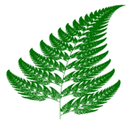
Likewise, in the fern frond below[2], one piece of the frond looks similar to the whole.
Similarly, if we zoom in on the coastline of Portugal[3], each zoom reveals previously hidden detail, and the coastline, while not identical to the view from further way, does exhibit similar characteristics.
Iterated Fractals
This self-similar behavior can be replicated through recursion: repeating a process over and over.
Example
Suppose that we start with a filled-in triangle. We connect the midpoints of each side and remove the middle triangle. We then repeat this process.
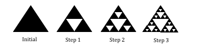
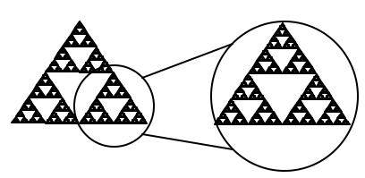
If we repeat this process, the shape that emerges is called the Sierpinski gasket. Notice that it exhibits self-similarity—any piece of the gasket will look identical to the whole. In fact, we can say that the Sierpinski gasket contains three copies of itself, each half as tall and wide as the original. Of course, each of those copies also contains three copies of itself.
In the following video, we present another explanation of how to generate a Sierpinski gasket using the idea of self-similarity.
We can construct other fractals using a similar approach. To formalize this a bit, we’re going to introduce the idea of initiators and generators.
Initiators and Generators
An initiator is a starting shape
A generator is an arranged collection of scaled copies of the initiator
To generate fractals from initiators and generators, we follow a simple rule:
Fractal Generation Rule
At each step, replace every copy of the initiator with a scaled copy of the generator, rotating as necessary
This process is easiest to understand through example.
Example
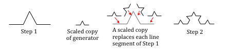
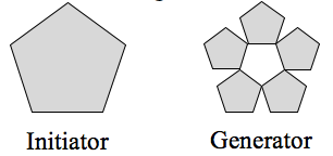
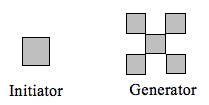
Use the initiator and generator shown to create the iterated fractal.

This tells us to, at each step, replace each line segment with the spiked shape shown in the generator. Notice that the generator itself is made up of 4 copies of the initiator. In step 1, the single line segment in the initiator is replaced with the generator. For step 2, each of the four line segments of step 1 is replaced with a scaled copy of the generator:
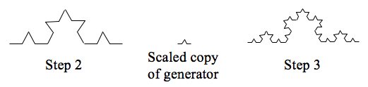
This process is repeated to form Step 3. Again, each line segment is replaced with a scaled copy of the generator.
Notice that since Step 0 only had 1 line segment, Step 1 only required one copy of Step 0.
Since Step 1 had 4 line segments, Step 2 required 4 copies of the generator.
Step 2 then had 16 line segments, so Step 3 required 16 copies of the generator.
Step 4, then, would require [latex]16\cdot4=64[/latex] copies of the generator.

The shape resulting from iterating this process is called the Koch curve, named for Helge von Koch who first explored it in 1904.
Notice that the Sierpinski gasket can also be described using the initiator-generator approach.
Example
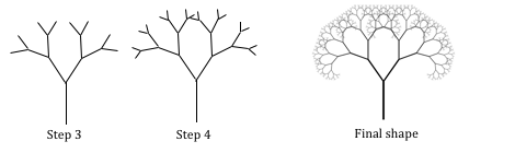
Use the initiator and generator below, however only iterate on the “branches.” Sketch several steps of the iteration.

We begin by replacing the initiator with the generator. We then replace each “branch” of Step 1 with a scaled copy of the generator to create Step 2.

Step 1, the generator. Step 2, one iteration of the generator.
We can repeat this process to create later steps. Repeating this process can create intricate tree shapes.[4]
Try It
Use the initiator and generator shown to produce the next two stages.

 |
 |
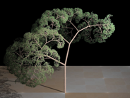
Using iteration processes like those above can create a variety of beautiful images evocative of nature.[5][6]
More natural shapes can be created by adding in randomness to the steps.
Example
Create a variation on the Sierpinski gasket by randomly skewing the corner points each time an iteration is made.
Suppose we start with the triangle below. We begin, as before, by removing the middle triangle. We then add in some randomness.
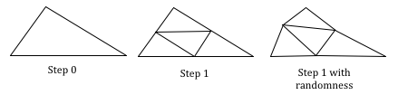
We then repeat this process.
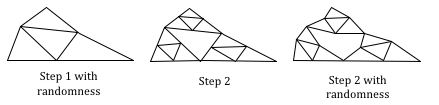
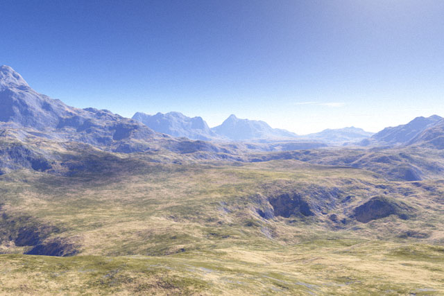
Continuing this process can create mountain-like structures. This landscape[7] was created using fractals, then colored and textured.
The following video provides another view of branching fractals, and randomness.
Fractal Dimension
In addition to visual self-similarity, fractals exhibit other interesting properties. For example, notice that each step of the Sierpinski gasket iteration removes one quarter of the remaining area. If this process is continued indefinitely, we would end up essentially removing all the area, meaning we started with a 2-dimensional area, and somehow end up with something less than that, but seemingly more than just a 1-dimensional line.
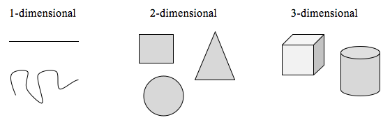
To explore this idea, we need to discuss dimension. Something like a line is 1-dimensional; it only has length. Any curve is 1-dimensional. Things like boxes and circles are 2-dimensional, since they have length and width, describing an area. Objects like boxes and cylinders have length, width, and height, describing a volume, and are 3-dimensional.
Certain rules apply for scaling objects, related to their dimension.
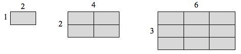
If I had a line with length 1, and wanted to scale its length by 2, I would need two copies of the original line. If I had a line of length 1, and wanted to scale its length by 3, I would need three copies of the original.
![]()
If I had a rectangle with length 2 and height 1, and wanted to scale its length and width by 2, I would need four copies of the original rectangle. If I wanted to scale the length and width by 3, I would need nine copies of the original rectangle.
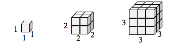
If I had a cubical box with sides of length 1, and wanted to scale its length and width by 2, I would need eight copies of the original cube. If I wanted to scale the length and width by 3, I would need 27 copies of the original cube.
Notice that in the 1-dimensional case, copies needed = scale.
In the 2-dimensional case, copies needed = scale[latex]^{2}[/latex].
In the 3-dimensional case, copies needed = scale[latex]^{3}[/latex].
From these examples, we might infer a pattern.
Scaling-Dimension Relation
To scale a D-dimensional shape by a scaling factor S, the number of copies C of the original shape needed will be given by:
[latex]\text{Copies}=\text{Scale}^{\text{Dimension}}[/latex], or [latex]C=S^{D}[/latex]
Example
Use the scaling-dimension relation to determine the dimension of the Sierpinski gasket.
Suppose we define the original gasket to have side length 1. The larger gasket shown is twice as wide and twice as tall, so has been scaled by a factor of 2.
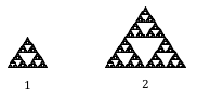
Notice that to construct the larger gasket, 3 copies of the original gasket are needed.
Using the scaling-dimension relation [latex]C=S^{D}[/latex], we obtain the equation [latex]3=2^{D}[/latex].
Since [latex]2^{1}=2[/latex] and [latex]2^{2}=4[/latex], we can immediately see that D is somewhere between 1 and 2; the gasket is more than a 1-dimensional shape, but we’ve taken away so much area its now less than 2-dimensional.
Solving the equation [latex]3=2^{D}[/latex] requires logarithms. If you studied logarithms earlier, you may recall how to solve this equation (if not, just skip to the box below and use that formula with the log key on a calculator):
Take the logarithm of both sides.
[latex]3={{2}^{D}}[/latex]
Use the exponent property of logs.
[latex]\log(3)=\log\left({{2}^{D}}\right)[/latex]
Divide by log(2).
[latex]\log(3)=D\log\left(2\right)[/latex]
The dimension of the gasket is about 1.585.
[latex]D=\frac{\log\left(3\right)}{\log(2)}\approx1.585[/latex]
Scaling-Dimension Relation, to find Dimension
To find the dimension D of a fractal, determine the scaling factor S and the number of copies C of the original shape needed, then use the formula
[latex]D=\frac{\log\left(C\right)}{\log(S)}[/latex]
Try It
Determine the fractal dimension of the fractal produced using the initiator and generator.

In the following video, we present a worked example of how to determine the dimension of the Sierpinski gasket
Candela Citations
- Introduction and Learning Outcomes. Provided by: Lumen Learning. License: CC BY: Attribution
- Revision and Adaptation. Provided by: Lumen Learning. License: CC BY: Attribution
- Question ID 131177. Authored by: Lumen Learning. License: CC BY: Attribution
- Iterated tree and twisted gasket. Authored by: OCLPhase2. Located at: https://youtu.be/OyAL-66GkJY. License: Public Domain: No Known Copyright
- Fractal dimension . Authored by: OCLPhase2. Located at: https://youtu.be/B1WTSsuDvWc. License: CC BY: Attribution
- http://en.wikipedia.org/wiki/File:Cauliflower_Fractal_AVM.JPG ↵
- http://www.flickr.com/photos/cjewel/3261398909/ ↵
- Openstreetmap.org, CC-BY-SA ↵
- http://www.flickr.com/photos/visualarts/5436068969/ ↵
- http://en.wikipedia.org/wiki/File:Fractal_tree_%28Plate_b_-_2%29.jpg ↵
- http://en.wikipedia.org/wiki/File:Barnsley_Fern_fractals_-_4_states.PNG ↵
- http://en.wikipedia.org/wiki/File:FractalLandscape.jpg ↵