Learning Objectives
- Graph linear functions using a table of values
- Graph a quadratic function using a table of values
- Identify important features of the graphs of a quadratic functions of the form [latex]f(x)=ax^2+bx+c[/latex]
- Graph a radical function using a table of values
- Identify how multiplication can change the graph of a radical function
- Identify how addition and subtraction can change the graph of a radical function
- Define one-to-one function
- Use the horizontal line test to determine whether a function is one-to-one
When both the input (independent variable) and the output (dependent variable) are real numbers, a function can be represented by a coordinate graph. The input is plotted on the horizontal x-axis and the output is plotted on the vertical y-axis.
A helpful first step in graphing a function is to make a table of values. This is particularly useful when you don’t know the general shape the function will have. You probably already know that a linear function will be a straight line, but let’s make a table first to see how it can be helpful.
When making a table, it’s a good idea to include negative values, positive values, and zero to ensure that you do have a linear function.
Make a table of values for [latex]f(x)=3x+2[/latex].
Make a two-column table. Label the columns x and f(x).
| x | f(x) |
|---|---|
Choose several values for x and put them as separate rows in the x column. These are YOUR CHOICE – there is no “right” or “wrong” values to pick, just go for it.
Tip: It’s always good to include 0, positive values, and negative values, if you can.
| x | f(x) |
|---|---|
| [latex]−2[/latex] | |
| [latex]−1[/latex] | |
| [latex]0[/latex] | |
| [latex]1[/latex] | |
| [latex]3[/latex] |
Evaluate the function for each value of x, and write the result in the f(x) column next to the x value you used.
When [latex]x=0[/latex], [latex]f(0)=3(0)+2=2[/latex],
[latex]f(1)=3(1)+2=5[/latex],
[latex]f(−1)=3(−1)+2=−3+2=−1[/latex], and so on.
| x | f(x) |
| [latex]−2[/latex] | [latex]−4[/latex] |
| [latex]−1[/latex] | [latex]−1[/latex] |
| [latex]0[/latex] | [latex]2[/latex] |
| [latex]1[/latex] | [latex]5[/latex] |
| [latex]3[/latex] | [latex]11[/latex] |
(Note that your table of values may be different from someone else’s. You may each choose different numbers for x.)
Now that you have a table of values, you can use them to help you draw both the shape and location of the function. Important: The graph of the function will show all possible values of x and the corresponding values of y. This is why the graph is a line and not just the dots that make up the points in our table.
Graph [latex]f(x)=3x+2[/latex].
Using the table of values we created above you can think of f(x) as y, each row forms an ordered pair that you can plot on a coordinate grid.
| x | f(x) |
| [latex]−2[/latex] | [latex]−4[/latex] |
| [latex]−1[/latex] | [latex]−1[/latex] |
| [latex]0[/latex] | [latex]2[/latex] |
| [latex]1[/latex] | [latex]5[/latex] |
| [latex]3[/latex] | [latex]11[/latex] |
Plot the points.

Since the points lie on a line, use a straight edge to draw the line. Try to go through each point without moving the straight edge.

Let’s try another one. Before you look at the answer, try to make the table yourself and draw the graph on a piece of paper.
Example
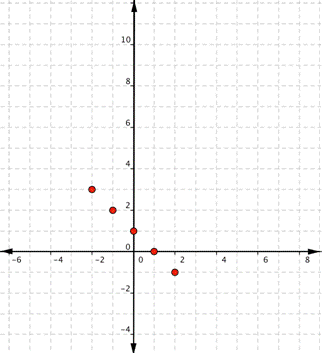
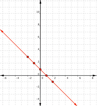
Graph [latex]f(x)=−x+1[/latex].
In the following video we show another example of how to graph a linear function on a set of coordinate axes.
These graphs are representations of a linear function. Remember that a function is a correspondence between two variables, such as x and y.
A General Note: Linear Function
A linear function is a function whose graph is a line. Linear functions can be written in the slope-intercept form of a line
[latex]f\left(x\right)=mx+b[/latex]
where [latex]b[/latex] is the initial or starting value of the function (when input, [latex]x=0[/latex]), and [latex]m[/latex] is the constant rate of change, or slope of the function. The y-intercept is at [latex]\left(0,b\right)[/latex]
Candela Citations
- Graph a Quadratic Function Using a Table of Value and the Vertex. Authored by: James Sousa (Mathispower4u.com) for Lumen Learning. Located at: https://youtu.be/leYhH_-3rVo. License: CC BY: Attribution
- Revision and Adaptation. Provided by: Lumen Learning. License: CC BY: Attribution
- Ex: Graph a Linear Function Using a Table of Values (Function Notation). Authored by: James Sousa (Mathispower4u.com) . Located at: https://youtu.be/sfzpdThXpA8. License: CC BY: Attribution
- Unit 17: Functions, from Developmental Math: An Open Program. Provided by: Monterey Institute of Technology and Education. Located at: http://nrocnetwork.org/dm-opentext. License: CC BY: Attribution
- Ex: Graph a Quadratic Function Using a Table of Values. Authored by: James Sousa (Mathispower4u.com) . Located at: https://youtu.be/wYfEzOJugS8. License: CC BY: Attribution
- Determine if a Relation Given as a Table is a One-to-One Function. Authored by: James Sousa (Mathispower4u.com) for Lumen Learning. Located at: https://youtu.be/QFOJmevha_Y. License: CC BY: Attribution
- Ex 1: Use the Vertical Line Test to Determine if a Graph Represents a Function. Authored by: James Sousa (Mathispower4u.com) . Located at: https://youtu.be/5Z8DaZPJLKY. License: CC BY: Attribution

