Learning Objectives
- Use an exponential model (when appropriate) to describe the relationship between two quantitative variables. Interpret the model in context.
Let’s summarize what we have learned about exponential growth models:
The general form of an exponential growth model is y = C · bx.
- C is the initial value. It is the y-value when x = 0. It is also the y-intercept.
- b is the growth factor; it will always be greater than 1 in cases of growth. From the growth factor, we can determine the percentage increase in y for each additional 1 unit increase in x.
Let’s compare the general form of an exponential growth model to the general form for a linear model: y = a + bx.
- In the linear model, a is the initial value. It is the y-value when x = 0. It is also the y-intercept.
- b is the slope. From the slope, we can determine the amount and direction the y-value changes for each additional 1 unit increase in x.
Now we apply what we have learned about exponential growth to find a model for a set of data.
In this activity, you use a simulation to find an exponential model that fits the population growth of Kenya.
Here are the data graphed in the scatterplot in the simulation.
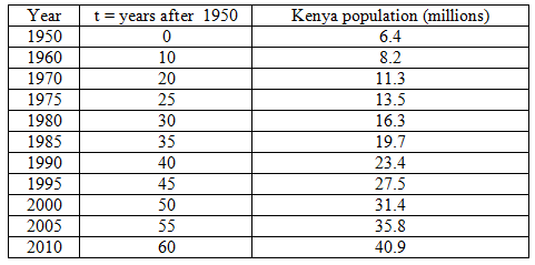
Notice that the Kenyan population growth has a strong positive exponential form. Use the sliders in the simulation to adjust the values of C and b to find a reasonable exponential model that fits this data.
Click here to open this simulation in its own window.
Learn By Doing
Candela Citations
- Concepts in Statistics. Provided by: Open Learning Initiative. Located at: http://oli.cmu.edu. License: CC BY: Attribution