Learning Objectives
- Describe the sampling distribution for sample proportions and use it to identify unusual (and more common) sample results.
- Distinguish between a sample statistic and a population parameter.
One of the goals of inference is to draw a conclusion about a population on the basis of a random sample from the population. Obviously, random samples vary, so we need to understand how much they vary and how they relate to the population. Our ultimate goal is to create a probability model that describes the long-run behavior of sample measurements. We use this model to make inferences about the population.
We begin our investigation with a simplified and artificial situation.
Example
Proportions from Random Samples Vary
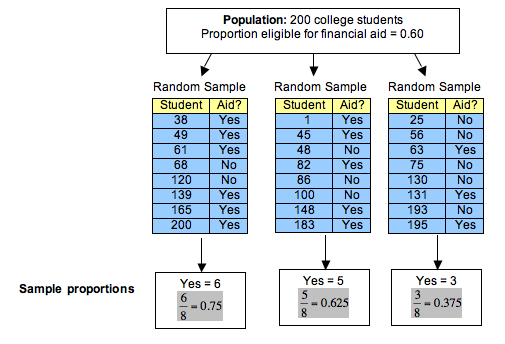
Imagine a small college with only 200 students, and suppose that 60% of these students are eligible for financial aid.
In this simplified situation, we can identify the population, the variable, and the population proportion.
- Population: 200 students at the college.
- Variable: Eligibility for financial aid is a categorical variable, so we use a proportion as a summary.
- Population proportion: 0.60 of the population is eligible for financial aid.
Note: Populations are usually much larger than 200 people. Also, in real situations, we do not know the population proportion. We are using a simplified situation to investigate how random samples relate to the population. This is the first step in creating a probability model that will be useful in inference.
How accurate are random samples at predicting this population proportion of 0.60?
To answer this question, we randomly select 8 students and determine the proportion who are eligible for financial aid. We repeat this process several times. Here are the results for 3 random samples:
Notice the following about these random samples:
- Each random sample came from a population in which the proportion eligible for financial aid is 0.60, but sample proportions vary. Each random sample has a different proportion who are eligible for financial aid.
- Some sample proportions are larger than the population proportion of 0.60; some sample proportions are smaller than the population proportion.
- Some samples give good estimates of the population proportion. Some do not. In this case, 0.625 is a much better estimate than 0.375.
- A lot of variability occurs in these sample proportions. It is not surprising, therefore, that a sample of 8 students may give an inaccurate estimate for the proportion of those eligible for financial aid in the population. It makes sense that small samples of only 8 students may not represent the population accurately. Later we investigate the effect of increasing the size of the sample.
- The variability we see in proportions from random samples is due to chance.
Learn By Doing
In these activites, we use the following simulation to select a random sample of 8 students from the small college in the previous example. At the college, 60% of the students are eligible for financial aid. For each sample, the simulation calculates the proportion in the sample who are eligible for financial aid. Repeat the sampling process many times to observe how the sample proportions vary, then answer the questions.
Click here to open this simulation in its own window.
Example
Means from Random Samples Vary
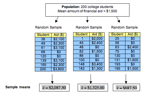
Now let’s consider a quantitative variable with this same population of 200 students at a small college. Let’s also suppose that the mean amount of financial aid received by students at the college is $1,500.
In this simplified situation, we have
- Population: 200 students at the college.
- Variable: Financial aid amount ($) is a quantitative variable, so we use a mean as a summary.
- Population mean: $1,500.
How accurate are random samples at predicting this population mean of $1,500?
To answer this question, we randomly select 8 students and determine the mean amount of financial aid received by the students. We repeat this process several times. Here are the results for 3 random samples:
Notice that observations we made earlier about sample proportions are true for sample means.
- Each random sample came from a population for which the mean amount of financial aid received by individual students is $1,500. But the sample means vary: Each random sample has a different mean.
- Some sample means are larger than the population mean of $1,500. Some sample means are smaller than the population mean.
- Some samples give better estimates of the population mean than others. For example, $1,325.00 is a much better estimate than $687.50.
- A lot of variability occurs in the sample means. It is not surprising, therefore, that a sample of 8 students may give an inaccurate estimate of the mean amount of financial aid received by the population. Again, it makes sense that small samples of only 8 students may not represent the population accurately. We investigate the factors that affect the variability of means from random samples in the module Inference for Means.
- The variability we see in the means from random samples is due to chance.
Definitions
Before we continue our discussion of sampling variability, we introduce some vocabulary.
A parameter is a number that describes a population. A statistic is a number that we calculate from a sample.
Let’s use this new vocabulary to rephrase what we already know at this point:
- When we do inference, the parameter is not known because it is impossible or impractical to gather data from everyone in the population. (Note: In each example on this page, we assumed we knew the parameter so that we could investigate how statistics relate to the parameter. This is the first step in creating a probability model. However, when we do inference, we use a statistic to draw a conclusion about an unknown parameter.)
- We make an inference about the population parameter on the basis of a sample statistic.
- Statistics from samples vary.
In this course, if the variable is categorical, the parameter and the statistic are both proportions. If the variable is quantitative, the parameter and statistic are both means.
From our first example:
- Parameter: A population proportion. For this population of students at a small college, 0.60 are eligible for financial aid.
- Statistics: Sample proportions that vary. In the example, 0.75, 0.625, and 0.375 are all statistics that describe the proportion eligible for financial aid in a sample of 8 students.
From our second example:
- Parameter: A population mean. For this population of students at a small college, the mean amount of financial aid is $1,500.
- Statistics: Sample means that vary. In the example, $2,087.50, $1,325.00, and $687.50 are all statistics that describe the mean amount of financial aid received by a sample of 8 students.
We use different notation for parameters and statistics:
| (Population) Parameter | (Sample) Statistic | |
|---|---|---|
| Proportion | [latex]p[/latex] | [latex]\stackrel{ˆ}{p}[/latex] |
| Mean | [latex]\mu[/latex] | [latex]\overline{x}[/latex] |
| Standard Deviation | [latex]\sigma[/latex] | [latex]s[/latex] |
Sometimes we refer to the sample statistics as “p-hat” and “x-bar.”
Here we use this notation for the information from our examples.
For our first example:
- For the population of college students, p = 0.60.
- For the 3 random samples of 8 students, we have p-hats [latex]\stackrel{ˆ}{p}=0.75,\text{}\stackrel{ˆ}{p}=0.625,\text{}\stackrel{ˆ}{p}=0.375[/latex]
For our second example:
- For the population of college students, µ = $1,500.
- For the 3 random samples of 8 students, we have x-bars [latex]\stackrel{¯}{x}=\$2,087.50,\text{}\stackrel{¯}{x}=\$1,325.00,\text{}\stackrel{¯}{x}=\$687.50[/latex]
Important Comments about Notation
Many statistics packages and introductory statistics textbooks use the notation shown in the table. The notation for means and standard deviations is common in the field of statistics. However, you will occasionally see other notation for proportions. In some statistical material, the Greek letter π represents the population proportion and p represents the sample proportion. This can be particularly confusing because p is used in some statistical material for the population proportion and in other statistical material for a sample proportion. Whenever you work with symbols, always be sure you understand what the symbol represents. You should be able to interpret the symbol from the context of the material.
Learn By Doing
Candela Citations
- Concepts in Statistics. Provided by: Open Learning Initiative. Located at: http://oli.cmu.edu. License: CC BY: Attribution