Learning Objectives
- Use mean and standard deviation to describe a distribution.
Introduction
In the section “Distributions for Quantitative Data,” we discussed the spread of a distribution in terms of a typical range of values. In “Quantifying Variability Relative to the Median,” we made this idea more precise with the interquartile range, IQR. The IQR gives us a measure of spread about the median. We defined a typical range of values about the median as the values between the first and third quartiles.
Now we want to develop a numerical measure of spread that we can use with the mean. In constructing a measure of spread about the mean, we want to compute how far a “typical” number is away from the mean.
Measuring Spread about the Mean
Let’s consider the sample data set 2, 2, 4, 5, 6, 7, 9. The mean of this data set is
[latex]\stackrel{¯}{x}=\frac{2+2+4+5+6+7+9\text{}}{7}\text{}=\text{}\frac{35}{7}=5[/latex]
Here is a dotplot of this data set with the mean marked by the vertical blue line.

We can see that some data is close to the mean and some data is further from the mean.
Since we want to see how the data points deviate from the mean, we determine how far each point is from the mean. We compute the difference between each of these values and the mean. These differences are called the deviations from the mean for each point.
| 2 − 5 = −3 |
| 2 − 5 = −3 |
| 4 − 5 = −1 |
| 5 − 5 = 0 |
| 6 − 5 = 1 |
| 7 − 5 = 2 |
| 9 − 5 = 4 |
When visualized on a dotplot, these differences are viewed as distances between each point and the mean. A negative difference indicates that the data point is to the left of the mean (shown in blue on the graph below). A positive difference indicates that the data point is to the right of the mean (shown in green on the graph below).

Our goal is to develop a single measurement that summarizes a typical distance from the mean. Before we continue, let’s practice determining the distance of a single data point from the mean.
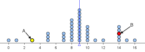
Learn By Doing
The two questions below refer to the following dotplot. The mean is 9 and it is marked by the vertical blue line.
Since we want to determine how far a typical number is away from the mean, we might try to average these numbers. However, if we add them all up, we will get 0 (try it). Getting 0 with this procedure (finding differences from mean and adding them all together) is no accident – it always produces 0. We have to overcome this problem.
Recall that we are trying to find the typical distance between data points and the mean. It therefore makes sense to take the absolute value of each of these differences.
| | 2 − 5 | = | −3 | = 3 |
| | 2 − 5 | = | −3 | = 3 |
| | 4 − 5 | = | −1 | = 1 |
| | 5 − 5 | = | 0 | = 0 |
| | 6 − 5 | = | 1 | = 1 |
| | 7 − 5 | = | 2 | = 2 |
| | 9 − 5 | = | 4 | = 4 |
Now we can compute the average of these deviations. There are seven data points, so we add these seven distances and divide by 7. The result is a measure of spread about the mean called the average deviation from the mean (ADM).
[latex]\frac{3+3+1+0+1+2+4\text{}}{7}\text{}=\text{}\frac{14}{7}=2[/latex]
We can indicate this average deviation on a dotplot with a graphic similar to a boxplot as follows.
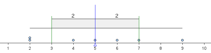
The shaded box in the middle is centered at the mean. It extends left and right a distance of 1 average deviation from the mean. Because the average deviation about the mean for this data set is 2, the box starts at 3 (because 5 − 2 = 3) and ends at 7 (because 5 + 2 = 7). In this way, we can use the ADM to define a typical range of values about the mean. Notice that this typical range of values (within 1 ADM of the mean) contains more than half of the values in the data set.
The goal of the next Learn By Doing exercise is to improve our intuition of what the ADM measures. We use the following simulation to investigate how the ADM responds to changes in a data set.
Instructions for adding or removing data points:
- To add a point, move the slider to the value you want, then click the + sign.
- To remove a point, move the slider to the value you want, then click the – sign.
- To reset the simulation to a blank screen, click the button in the upper left corner that says Reset.
Click here to open this simulation in its own window.
Learn By Doing
Learn By Doing
Before we continue, let’s summarize our main points:
- The ADM (average distance from the mean) is a measurement of spread about the mean. More precisely, ADM measures the average distance of the data from the mean.
- We can use the ADM to define a typical range of values about the mean. We mark the mean, then we mark 1 ADM below the mean and 1 ADM above the mean. This interval is centered at the mean and captures typical values about the mean.
Using these two ideas, we can estimate the ADM by looking at a graph of the distribution of data. We practice this important skill in the next Learn By Doing.
Learn By Doing
In the next example, we compare the ADM as a measure of spread to the other ways we have measured spread.
Example
Measuring Variability in Different Ways
The following dotplots show the potassium content in 76 cereals. Compare children’s cereals to adult cereals. Which type of cereal has more variability in potassium content?
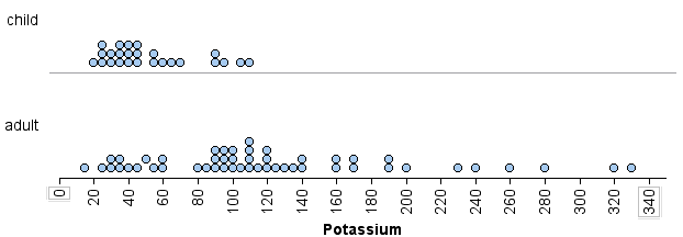
We can visually see that there is more variability in the potassium content of the adult cereals than in the children’s cereals. We can measure this spread in three ways:
- Using overall range: The range of potassium content is larger for the adult cereals than for the children’s cereals. The children’s cereal set has a range of 90 (because 110 − 20 = 90), whereas the adult cereal set has a range of 315 (because 330 − 15 = 315).
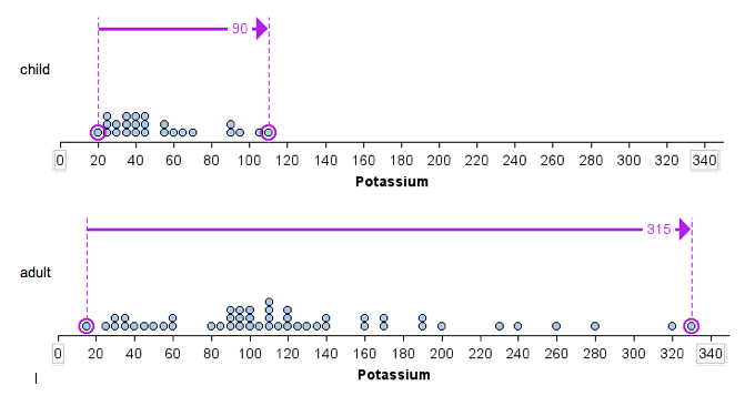
- Using IQR: The IQR of the adult cereal set is larger than the IQR of the children’s cereal set. The adult cereal set has an IQR of 80, since for that set Q1 = 80 and Q3 = 160. The children’s cereal set has an IQR of 30, since for that set Q1 = 35 and Q3 = 65. Notice here we use the median as a measure of center. The median is marked with a red line. IQR measures spread about the median.

- Using ADM: The children’s cereal data set has an ADM of 22. The adult cereal data set has an ADM of 55. Notice here we use the mean as a measure of center. The mean is marked with a blue line. ADM measures spread about the mean.
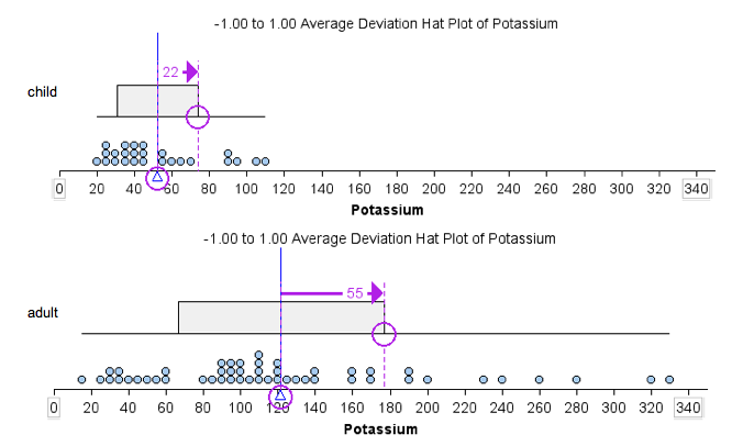
Based on the preceding example, we might expect the data set with the larger range to also have the larger ADM. This is not true, as we illustrate in the next example.
Example
Comparing Range and ADM
Which data set has more variability? Our answer to this question depends on how we measure variability.

We can see that the overall range is larger for data set b.
- Data set a: range = 100 − 0 = 100
- Data set b: range = 200 − 0 = 200
If we use overall range to measure spread, we will say that data set b has more variability.
Does our answer change if we use ADM to measure spread? Yes!
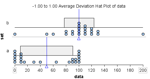
- Data set a: ADM = 41
- Data set b: ADM = 23
Most of the data in data set a is located away from the mean, so the ADM is large: 41. Compare this to data set b. Most of the data in data set b is located close to the mean, so the ADM is small: 23.
If we use ADM as a measure of spread, we will say that data set a has more variability.
The ADM is a reasonable measure of spread about the mean, but there is another measure that is used much more often: the standard deviation (SD). The standard deviation behaves very much like the average deviation. So all of the work we have done on this page is useful in understanding standard deviation. We discuss standard deviation next.
Candela Citations
- Concepts in Statistics. Provided by: Open Learning Initiative. Located at: http://oli.cmu.edu. License: CC BY: Attribution