Definition of a Limit

Learning Outcomes

Using correct notation, describe the limit of a function
Use a table of values to estimate the limit of a function or to identify when the limit does not exist
Use a graph to estimate the limit of a function or to identify when the limit does not exist

We begin our exploration of limits by taking a look at the graphs of the functions

f (x) = \frac{x^{2} - 4}{x - 2}, g (x) = \frac{| x - 2 |}{x - 2}

$f(x)=\dfrac{x^2-4}{x-2}, \ \, g(x)=\dfrac{|x-2|}{x-2}$ , and

h (x) = \frac{1}{(x - 2)^{2}}

$h(x)=\dfrac{1}{(x-2)^2}$ ,

which are shown in Figure 1. In particular, let’s focus our attention on the behavior of each graph at and around $x=2$ .

"Three 2 and x= -1 for x < 2. There are open circles at both endpoints (2, 1) and (-2, 1). The third is h(x) = 1 / (x-2)^2, in which the function curves asymptotically towards y=0 and x=2 in quadrants one and two." width="975" height="434"

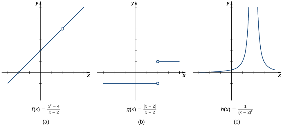
Figure 1. These graphs show the behavior of three different functions around $x=2$ .

Each of the three functions is undefined at $x=2$ , but if we make this statement and no other, we give a very incomplete picture of how each function behaves in the vicinity of $x=2$ . To express the behavior of each graph in the vicinity of 2 more completely, we need to introduce the concept of a limit.

Intuitive Definition of a Limit

Let’s first take a closer look at how the function $f(x)=\dfrac{(x^2-4)}{(x-2)}$ behaves around $x=2$ in Figure 1. As the values of $x$ approach 2 from either side of 2, the values of $y=f(x)$ approach 4. Mathematically, we say that the limit of $f(x)$ as $x$ approaches 2 is 4. Symbolically, we express this limit as

lim x \to 2 f (x) = 4

$\underset{x \to 2}{\lim}f(x)=4$

From this very brief informal look at one limit, let’s start to develop an intuitive definition of the limit. We can think of the limit of a function at a number $a$ as being the one real number $L$ that the functional values approach as the $x$ -values approach $a$ , provided such a real number $L$ exists. Stated more carefully, we have the following definition:

Definition

Let $f(x)$ be a function defined at all values in an open interval containing $a$ , with the possible exception of $a$ itself, and let $L$ be a real number. If all values of the function $f(x)$ approach the real number $L$ as the values of $x(\ne a)$ approach the number $a$ , then we say that the limit of $f(x)$ as $x$ approaches $a$ is $L$ . (More succinct, as $x$ gets closer to $a$ , $f(x)$ gets closer and stays close to $L$ .) Symbolically, we express this idea as

lim x \to a f (x) = L

$\underset{x\to a}{\lim}f(x)=L$

Try It

We can estimate limits by constructing tables of functional values and by looking at their graphs. This process is described in the following Problem-Solving Strategy.

Problem-Solving Strategy: Evaluating a Limit Using a Table of Functional Values

To evaluate

lim x \to a f (x)

$\underset{x\to a}{\lim}f(x)$ , we begin by completing a table of functional values. We should choose two sets of

x

$x$ -values—one set of values approaching

a

$a$ and less than

a

$a$ , and another set of values approaching

a

$a$ and greater than

a

$a$ . The table below demonstrates what your tables might look like.

Table of Functional Values for $\underset{x\to a}{\lim}f(x)$
$x$	$f(x)$	$x$	$f(x)$
$a-0.1$	$f(a-0.1)$	$a+0.1$	$f(a+0.1)$
$a-0.01$	$f(a-0.01)$	$a+0.01$	$f(a+0.01)$
$a-0.001$	$f(a-0.001)$	$a+0.001$	$f(a+0.001)$
$a-0.0001$	$f(a-0.0001)$	$a+0.0001$	$f(a+0.0001)$
Use additional values as necessary.		Use additional values as necessary.

Next, let’s look at the values in each of the $f(x)$ columns and determine whether the values seem to be approaching a single value as we move down each column. In our columns, we look at the sequence $f(a-0.1), \, f(a-0.01), \, f(a-0.001), \, f(a-0.0001),$ and so on, and $f(a+0.1), \, f(a+0.01), \, f(a+0.001), \, f(a+0.0001)$ and so on. (Note: Although we have chosen the $x$ -values $a \pm 0.1, \, a \pm 0.01, \, a \pm 0.001, \, a \pm 0.0001$ , and so forth, and these values will probably work nearly every time, on very rare occasions we may need to modify our choices.)
If both columns approach a common $y$ -value $L$ , we state $\underset{x\to a}{\lim}f(x)=L$ . We can use the following strategy to confirm the result obtained from the table or as an alternative method for estimating a limit.
Using a graphing calculator or computer software that allows us graph functions, we can plot the function $f(x)$ , making sure the functional values of $f(x)$ for $x$ -values near $a$ are in our window. We can use the trace feature to move along the graph of the function and watch the $y$ -value readout as the $x$ -values approach $a$ . If the $y$ -values approach $L$ as our $x$ -values approach $a$ from both directions, then $\underset{x\to a}{\lim}f(x)=L$ . We may need to zoom in on our graph and repeat this process several times.

We apply this Problem-Solving Strategy to compute a limit below.

Example: Evaluating a Limit Using a Table of Functional Values 1

Evaluate $\underset{x\to 0}{\lim}\dfrac{\sin x}{x}$ using a table of functional values.

Show Solution

We have calculated the values of

f (x) = \frac{(sin x)}{x}

$f(x)=\dfrac{(\sin x)}{x}$ for the values of

x

$x$ listed in the table below.

Table of Functional Values for $\underset{x\to 0}{\lim}\frac{\sin x}{x}$
$x$	$\frac{\sin x}{x}$	$x$	$\frac{\sin x}{x}$
−0.1	0.998334166468	0.1	0.998334166468
−0.01	0.999983333417	0.01	0.999983333417
−0.001	0.999999833333	0.001	0.999999833333
−0.0001	0.999999998333	0.0001	0.999999998333

Note: The values in this table were obtained using a calculator and using all the places given in the calculator output.

As we read down each $\frac{\sin x}{x}$ column, we see that the values in each column appear to be approaching one. Thus, it is fairly reasonable to conclude that $\underset{x\to 0}{\lim}\frac{\sin x}{x}=1$ . A calculator-or computer-generated graph of $f(x)=\frac{\sin x}{x}$ would be similar to that shown in Figure 2, and it confirms our estimate.

A graph of f(x) = sin(x)/x over the interval [-6, 6]. The curving function has a y intercept at x=0 and x intercepts at y=pi and y=-pi.

Figure 2. The graph of $f(x)=(\sin x)/x$ confirms the estimate from the table.

Example: Evaluating a Limit Using a Table of Functional Values 2

Evaluate $\underset{x\to 4}{\lim}\dfrac{\sqrt{x}-2}{x-4}$ using a table of functional values.

Show Solution

As before, we use a table to list the values of the function for the given values of $x$ .

Table of Functional Values for $\underset{x\to 4}{\lim}\frac{\sqrt{x}-2}{x-4}$
$x$	$\frac{\sqrt{x}-2}{x-4}$	$x$	$\frac{\sqrt{x}-2}{x-4}$
3.9	0.251582341869	4.1	0.248456731317
3.99	0.25015644562	4.01	0.24984394501
3.999	0.250015627	4.001	0.249984377
3.9999	0.250001563	4.0001	0.249998438
3.99999	0.25000016	4.00001	0.24999984

After inspecting this table, we see that the functional values less than 4 appear to be decreasing toward 0.25 whereas the functional values greater than 4 appear to be increasing toward 0.25. We conclude that $\underset{x\to 4}{\lim}\frac{\sqrt{x}-2}{x-4}=0.25$ . We confirm this estimate using the graph of $f(x)=\frac{\sqrt{x}-2}{x-4}$ shown in Figure 3.

A graph of the function f(x) = (sqrt(x) – 2 ) / (x-4) over the interval [0,8]. There is an open circle on the function at x=4. The function curves asymptotically towards the x axis and y axis in quadrant one.

Figure 3. The graph of $f(x)=\frac{\sqrt{x}-2}{x-4}$ confirms the estimate from the table.

Try It

Estimate $\underset{x\to 1}{\lim}\dfrac{\frac{1}{x}-1}{x-1}$ using a table of functional values. Use a graph to confirm your estimate.

Hint

Show Solution

$\underset{x\to 1}{\lim}\frac{\frac{1}{x}-1}{x-1}=-1$

Try It

At this point, we see from the tables that it may be just as easy, if not easier, to estimate a limit of a function by inspecting its graph as it is to estimate the limit by using a table of functional values. In the example below, we evaluate a limit exclusively by looking at a graph rather than by using a table of functional values. Recall that looking at a graph, a function’s value at a given x value is simply the y value at x.

Example: Evaluating a Limit Using a Graph

For $g(x)$ shown in Figure 4, evaluate $\underset{x\to -1}{\lim}g(x)$ .

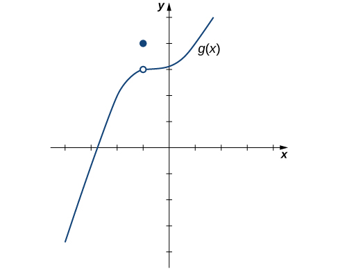
The graph of a generic curving function g(x). In quadrant two, there is an open circle on the function at (-1,3) and a closed circle one unit up at (-1, 4).

Figure 4. The graph of $g(x)$ includes one value not on a smooth curve.

Show Solution

Despite the fact that $g(-1)=4$ , as the $x$ -values approach −1 from either side, the $g(x)$ values approach 3. Therefore, $\underset{x\to -1}{\lim}g(x)=3$ . Note that we can determine this limit without even knowing the algebraic expression of the function.

Based on the example above, we make the following observation: It is possible for the limit of a function to exist at a point, and for the function to be defined at this point, but the limit of the function and the value of the function at the point may be different.

Watch the following video to see the more examples of evaluating a limit using a graph

Closed Captioning and Transcript Information for Video

Try It

Use the graph of $h(x)$ in Figure 5 to evaluate $\underset{x\to 2}{\lim}h(x)$ , if possible.

A graph of the function h(x), which is a parabola graphed over [-2.5, 5]. There is an open circle where the vertex should be at the point (2,-1).

Figure 5. The graph of $h(x)$ consists of a smooth graph with a single removed point at $x=2$ .

Hint

What $y$ -value does the function approach as the $x$ -values approach 2?

Show Solution

$\underset{x\to 2}{\lim}h(x)=-1$ .

Looking at a table of functional values or looking at the graph of a function provides us with useful insight into the value of the limit of a function at a given point. However, these techniques rely too much on guesswork. We eventually need to develop alternative methods of evaluating limits. These new methods are more algebraic in nature and we explore them in the next section; however, at this point we introduce two special limits that are foundational to the techniques to come.

Two Important Limits

Let $a$ be a real number and $c$ be a constant.

$\underset{x\to a}{\lim}x=a$
$\underset{x\to a}{\lim}c=c$

We can make the following observations about these two limits.

For the first limit, observe that as $x$ approaches $a$ , so does $f(x)$ , because $f(x)=x$ . Consequently, $\underset{x\to a}{\lim}x=a$ .
For the second limit, consider the table below.

Table of Functional Values for $\underset{x\to a}{\lim}c=c$
$x$	$f(x)=c$	$x$	$f(x)=c$
$a-0.1$	$c$	$a+0.1$	$c$
$a-0.01$	$c$	$a+0.01$	$c$
$a-0.001$	$c$	$a+0.001$	$c$
$a-0.0001$	$c$	$a+0.0001$	$c$

Observe that for all values of $x$ (regardless of whether they are approaching $a$ ), the values $f(x)$ remain constant at $c$ . We have no choice but to conclude $\underset{x\to a}{\lim}c=c$ .

The Existence of a Limit

As we consider the limit in the next example, keep in mind that for the limit of a function to exist at a point, the functional values must approach a single real-number value at that point. If the functional values do not approach a single value, then the limit does not exist.

Example: Evaluating a Limit That Fails to Exist

Evaluate $\underset{x\to 0}{\lim} \sin \left(\dfrac{1}{x}\right)$ using a table of values.

Show Solution

The table below lists values for the function $\sin \left(\dfrac{1}{x}\right)$ for the given values of $x$ .

Table of Functional Values for $\underset{x\to 0}{\lim} \sin (\frac{1}{x})$
$x$	$\sin (\frac{1}{x})$	$x$	$\sin (\frac{1}{x})$
−0.1	0.544021110889	0.1	−0.544021110889
−0.01	0.50636564111	0.01	−0.50636564111
−0.001	−0.8268795405312	0.001	0.826879540532
−0.0001	0.305614388888	0.0001	−0.305614388888
−0.00001	−0.035748797987	0.00001	0.035748797987
−0.000001	0.349993504187	0.000001	−0.349993504187

After examining the table of functional values, we can see that the $y$ -values do not seem to approach any one single value. It appears the limit does not exist. Before drawing this conclusion, let’s take a more systematic approach. Take the following sequence of $x$ -values approaching 0:

$\frac{2}{\pi }, \, \frac{2}{3\pi }, \, \frac{2}{5\pi }, \, \frac{2}{7\pi }, \, \frac{2}{9\pi }, \, \frac{2}{11\pi }, \, \cdots$

The corresponding $y$ -values are

$1, \, -1, \, 1, \, -1, \, 1, \, -1, \, \cdots$

At this point we can indeed conclude that $\underset{x\to 0}{\lim} \sin (\frac{1}{x})$ does not exist.

Mathematicians frequently abbreviate “does not exist” as DNE.

Thus, we would write $\underset{x\to 0}{\lim} \sin (\frac{1}{x})$ DNE.) The graph of $f(x)= \sin (\frac{1}{x})$ is shown in Figure 6 and it gives a clearer picture of the behavior of $\sin (\frac{1}{x})$ as $x$ approaches 0. You can see that $\sin (\frac{1}{x})$ oscillates ever more wildly between −1 and 1 as $x$ approaches 0.

The graph of the function f(x) = sin(1/x), which oscillates rapidly between -1 and 1 as x approaches 0. The oscillations are less frequent as the function moves away from 0 on the x axis.

Figure 6. The graph of $f(x)= \sin (\frac{1}{x})$ oscillates rapidly between −1 and 1 as x approaches 0.

Try It

Use a table of functional values to evaluate $\underset{x\to 2}{\lim}\dfrac{|x^2-4|}{x-2}$ , if possible.

Hint

Use $x$ -values 1.9, 1.99, 1.999, 1.9999, 1.9999 and 2.1, 2.01, 2.001, 2.0001, 2.00001 in your table.

Show Solution

$\underset{x\to 2}{\lim}\frac{|x^2-4|}{x-2}$ does not exist.

Module 2: Limits