Computing Differentials

We have seen that linear approximations can be used to estimate function values. They can also be used to estimate the amount a function value changes as a result of a small change in the input. To discuss this more formally, we define a related concept: differentials. Differentials provide us with a way of estimating the amount a function changes as a result of a small change in input values.

When we first looked at derivatives, we used the Leibniz notation [latex]dy/dx[/latex] to represent the derivative of [latex]y[/latex] with respect to [latex]x[/latex]. Although we used the expressions [latex]dy[/latex] and [latex]dx[/latex] in this notation, they did not have meaning on their own. Here we see a meaning to the expressions [latex]dy[/latex] and [latex]dx[/latex]. Suppose [latex]y=f(x)[/latex] is a differentiable function. Let [latex]dx[/latex] be an independent variable that can be assigned any nonzero real number, and define the dependent variable [latex]dy[/latex] by

It is important to notice that [latex]dy[/latex] is a function of both [latex]x[/latex] and [latex]dx[/latex]. The expressions [latex]dy[/latex] and [latex]dx[/latex] are called differentials. We can divide both sides of the equation by [latex]dx[/latex], which yields

This is the familiar expression we have used to denote a derivative. The first equation is known as the differential form of the second one.

Watch the following video to see the worked solution to Example: Computing differentials.

We now connect differentials to linear approximations. Differentials can be used to estimate the change in the value of a function resulting from a small change in input values. Consider a function [latex]f[/latex] that is differentiable at point [latex]a[/latex]. Suppose the input [latex]x[/latex] changes by a small amount. We are interested in how much the output [latex]y[/latex] changes. If [latex]x[/latex] changes from [latex]a[/latex] to [latex]a+dx[/latex], then the change in [latex]x[/latex] is [latex]dx[/latex] (also denoted [latex]\Delta x[/latex]), and the change in [latex]y[/latex] is given by

Instead of calculating the exact change in [latex]y[/latex], however, it is often easier to approximate the change in [latex]y[/latex] by using a linear approximation. For [latex]x[/latex] near [latex]a[/latex], [latex]f(x)[/latex] can be approximated by the linear approximation

Therefore, if [latex]dx[/latex] is small,

That is,

In other words, the actual change in the function [latex]f[/latex] if [latex]x[/latex] increases from [latex]a[/latex] to [latex]a+dx[/latex] is approximately the difference between [latex]L(a+dx)[/latex] and [latex]f(a)[/latex], where [latex]L(x)[/latex] is the linear approximation of [latex]f[/latex] at [latex]a[/latex]. By definition of [latex]L(x)[/latex], this difference is equal to [latex]f^{\prime}(a)dx[/latex]. In summary,

Therefore, we can use the differential [latex]dy=f^{\prime}(a) \, dx[/latex] to approximate the change in [latex]y[/latex] if [latex]x[/latex] increases from [latex]x=a[/latex] to [latex]x=a+dx[/latex]. We can see this in the following graph.

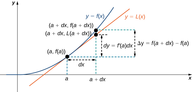
Figure 5. The differential [latex]dy=f^{\prime}(a) \, dx[/latex] is used to approximate the actual change in [latex]y[/latex] if [latex]x[/latex] increases from [latex]a[/latex] to [latex]a+dx[/latex].

We now take a look at how to use differentials to approximate the change in the value of the function that results from a small change in the value of the input. Note the calculation with differentials is much simpler than calculating actual values of functions and the result is very close to what we would obtain with the more exact calculation.

Calculating the Amount of Error

Any type of measurement is prone to a certain amount of error. In many applications, certain quantities are calculated based on measurements. For example, the area of a circle is calculated by measuring the radius of the circle. An error in the measurement of the radius leads to an error in the computed value of the area. Here we examine this type of error and study how differentials can be used to estimate the error.

Consider a function [latex]f[/latex] with an input that is a measured quantity. Suppose the exact value of the measured quantity is [latex]a[/latex], but the measured value is [latex]a+dx[/latex]. We say the measurement error is [latex]dx[/latex] (or [latex]\Delta x[/latex]). As a result, an error occurs in the calculated quantity [latex]f(x)[/latex]. This type of error is known as a propagated error and is given by

Since all measurements are prone to some degree of error, we do not know the exact value of a measured quantity, so we cannot calculate the propagated error exactly. However, given an estimate of the accuracy of a measurement, we can use differentials to approximate the propagated error [latex]\Delta y[/latex]. Specifically, if [latex]f[/latex] is a differentiable function at [latex]a[/latex], the propagated error is

Unfortunately, we do not know the exact value [latex]a[/latex]. However, we can use the measured value [latex]a+dx[/latex], and estimate

In the next example, we look at how differentials can be used to estimate the error in calculating the volume of a box if we assume the measurement of the side length is made with a certain amount of accuracy.

Watch the following video to see the worked solution to Example: Volume of a Cube.

The measurement error [latex]dx \, (=\Delta x)[/latex] and the propagated error [latex]\Delta y[/latex] are absolute errors. We are typically interested in the size of an error relative to the size of the quantity being measured or calculated. Given an absolute error [latex]\Delta q[/latex] for a particular quantity, we define the relative error as [latex]\frac{\Delta q}{q}[/latex], where [latex]q[/latex] is the actual value of the quantity. The percentage error is the relative error expressed as a percentage. For example, if we measure the height of a ladder to be 63 in. when the actual height is 62 in., the absolute error is 1 in. but the relative error is [latex]\frac{1}{62}=0.016[/latex], or [latex]1.6 \%[/latex]. By comparison, if we measure the width of a piece of cardboard to be 8.25 in. when the actual width is 8 in., our absolute error is [latex]\frac{1}{4}[/latex] in., whereas the relative error is [latex]\frac{0.25}{8}=\frac{1}{32}[/latex], or [latex]3.1\%[/latex]. Therefore, the percentage error in the measurement of the cardboard is larger, even though 0.25 in. is less than 1 in.