Linear Approximation of a Function at a Point

Learning Outcomes

Describe the linear approximation to a function at a point.
Write the linearization of a given function.

Consider a function $f$ that is differentiable at a point $x=a$ . Recall that the tangent line to the graph of $f$ at $a$ is given by the equation

y = f (a) + f^{'} (a) (x - a)

$y=f(a)+f^{\prime}(a)(x-a)$

This is simply derived from the point-slope form of the equation of a line $y-{y}_{1}=m\left(x-{x}_{1}\right)$ by adding ${y}_{1}$ to both sides!

For example, consider the function $f(x)=\frac{1}{x}$ at $a=2$ . Since $f$ is differentiable at $x=2$ and $f^{\prime}(x)=-\frac{1}{x^2}$ , we see that $f^{\prime}(2)=-\frac{1}{4}$ . Therefore, the tangent line to the graph of $f$ at $a=2$ is given by the equation

y = \frac{1}{2} - \frac{1}{4} (x - 2)

$y=\dfrac{1}{2}-\dfrac{1}{4}(x-2)$

Figure 1a shows a graph of $f(x)=\frac{1}{x}$ along with the tangent line to $f$ at $x=2$ . Note that for $x$ near 2, the graph of the tangent line is close to the graph of $f$ . As a result, we can use the equation of the tangent line to approximate $f(x)$ for $x$ near 2. For example, if $x=2.1$ , the $y$ value of the corresponding point on the tangent line is

y = \frac{1}{2} - \frac{1}{4} (2.1 - 2) = 0.475

$y=\dfrac{1}{2}-\dfrac{1}{4}(2.1-2)=0.475$

The actual value of $f(2.1)$ is given by

f (2.1) = \frac{1}{2.1} \approx 0.47619

$f(2.1)=\dfrac{1}{2.1}\approx 0.47619$

Therefore, the tangent line gives us a fairly good approximation of $f(2.1)$ (Figure 1b). However, note that for values of $x$ far from 2, the equation of the tangent line does not give us a good approximation. For example, if $x=10$ , the $y$ -value of the corresponding point on the tangent line is

y = \frac{1}{2} - \frac{1}{4} (10 - 2) = \frac{1}{2} - 2 = - 1.5

$y=\frac{1}{2}-\dfrac{1}{4}(10-2)=\dfrac{1}{2}-2=-1.5$ ,

whereas the value of the function at $x=10$ is $f(10)=0.1$ .

This figure has two parts a and b. In figure a, the line f(x) = 1/x is shown with its tangent line at x = 2. In figure b, the area near the tangent point is blown up to show how good of an approximation the tangent is near x = 2.

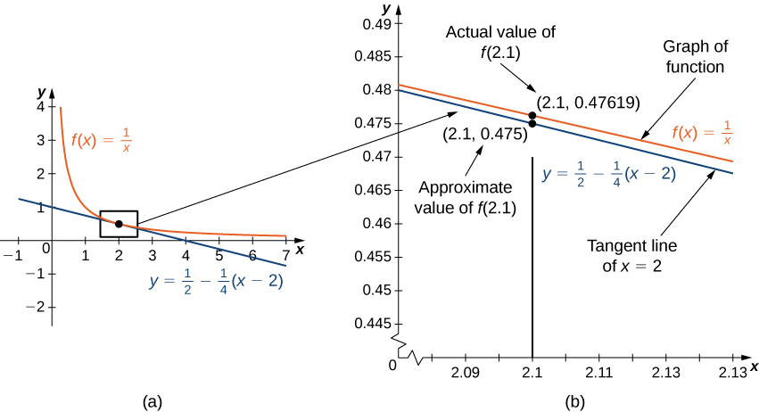
Figure 1. (a) The tangent line to $f(x)=\frac{1}{x}$ at $x=2$ provides a good approximation to $f$ for $x$ near 2. (b) At $x=2.1$ , the value of $y$ on the tangent line to $f(x)=\frac{1}{x}$ is 0.475. The actual value of $f(2.1)$ is $\frac{1}{2.1}$ , which is approximately 0.47619.

In general, for a differentiable function $f$ , the equation of the tangent line to $f$ at $x=a$ can be used to approximate $f(x)$ for $x$ near $a$ . Therefore, we can write

f (x) \approx f (a) + f^{'} (a) (x - a)

$f(x)\approx f(a)+f^{\prime}(a)(x-a)$ for

x

$x$ near

a

$a$

We call the linear function

L (x) = f (a) + f^{'} (a) (x - a)

$L(x)=f(a)+f^{\prime}(a)(x-a)$

the linear approximation, or tangent line approximation, of $f$ at $x=a$ . This function $L$ is also known as the linearization of $f$ at $x=a$ .

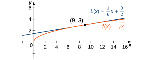
To show how useful the linear approximation can be, we look at how to find the linear approximation for $f(x)=\sqrt{x}$ at $x=9$ .

Example: Linear Approximation of $\sqrt{x}$

Find the linear approximation of $f(x)=\sqrt{x}$ at $x=9$ and use the approximation to estimate $\sqrt{9.1}$ .

Show Solution

Since we are looking for the linear approximation at $x=9$ , using the tangent line approximation, we know the linear approximation is given by

L (x) = f (9) + f^{'} (9) (x - 9)

$L(x)=f(9)+f^{\prime}(9)(x-9)$ .

We need to find $f(9)$ and $f^{\prime}(9)$ .

\begin{matrix} f (x) = \sqrt{x} & \Rightarrow & f (9) = \sqrt{9} = 3 f^{'} (x) = \frac{1}{2 \sqrt{x}} & \Rightarrow & f^{'} (9) = \frac{1}{2 \sqrt{9}} = \frac{1}{6} \end{matrix}

$\begin{array}{lll} f(x)=\sqrt{x}& \Rightarrow & f(9)=\sqrt{9}=3 \\ f^{\prime}(x)=\frac{1}{2\sqrt{x}}& \Rightarrow & f^{\prime}(9)=\frac{1}{2\sqrt{9}}=\frac{1}{6} \end{array}$

Therefore, the linear approximation is given by Figure 2.

L (x) = 3 + \frac{1}{6} (x - 9)

$L(x)=3+\frac{1}{6}(x-9)$

Using the linear approximation, we can estimate $\sqrt{9.1}$ by writing

\sqrt{9.1} = f (9.1) \approx L (9.1) = 3 + \frac{1}{6} (9.1 - 9) \approx 3.0167

$\sqrt{9.1}=f(9.1)\approx L(9.1)=3+\frac{1}{6}(9.1-9)\approx 3.0167$ .

The function f(x) = the square root of x is shown with its tangent at (9, 3). The tangent appears to be a very good approximation from x = 6 to x = 12.

Figure 2. The local linear approximation to $f(x)=\sqrt{x}$ at $x=9$ provides an approximation to $f$ for $x$ near 9.

Analysis

Using a calculator, the value of $\sqrt{9.1}$ to four decimal places is 3.0166. The value given by the linear approximation, 3.0167, is very close to the value obtained with a calculator, so it appears that using this linear approximation is a good way to estimate $\sqrt{x}$ , at least for $x$ near 9. At the same time, it may seem odd to use a linear approximation when we can just push a few buttons on a calculator to evaluate $\sqrt{9.1}$ . However, how does the calculator evaluate $\sqrt{9.1}$ ? The calculator uses an approximation! In fact, calculators and computers use approximations all the time to evaluate mathematical expressions; they just use higher-degree approximations.

Watch the following video to see the worked solution to Example: Linear Approximation of $\sqrt{x}$ .

Closed Captioning and Transcript Information for Video

Try It

Find the local linear approximation to $f(x)=\sqrt[3]{x}$ at $x=8$ . Use it to approximate $\sqrt[3]{8.1}$ to five decimal places.

Hint

$L(x)=f(a)+f^{\prime}(a)(x-a)$

Show Solution

$L(x)=2+\frac{1}{12}(x-8)$ ; 2.00833

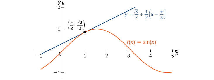
Example: Linear Approximation of $\sin x$

Find the linear approximation of $f(x)= \sin x$ at $x=\dfrac{\pi}{3}$ and use it to approximate $\sin (62^{\circ})$ .

Show Solution

First we note that since $\frac{\pi}{3}$ rad is equivalent to $60^{\circ}$ , using the linear approximation at $x=\pi /3$ seems reasonable. The linear approximation is given by

L (x) = f (\frac{π}{3}) + f^{'} (\frac{π}{3}) (x - \frac{π}{3})

$L(x)=f(\frac{\pi}{3})+f^{\prime}(\frac{\pi}{3})(x-\frac{\pi}{3})$ .

We see that

\begin{matrix} f (x) = sin x & \Rightarrow & f (\frac{π}{3}) = sin (\frac{π}{3}) = \frac{\sqrt{3}}{2} f^{'} (x) = cos x & \Rightarrow & f^{'} (\frac{π}{3}) = cos (\frac{π}{3}) = \frac{1}{2} \end{matrix}

$\begin{array}{lll}f(x)= \sin x & \Rightarrow & f(\frac{\pi}{3})= \sin (\frac{\pi}{3})=\frac{\sqrt{3}}{2} \\ f^{\prime}(x)= \cos x & \Rightarrow & f^{\prime}(\frac{\pi}{3})= \cos (\frac{\pi}{3})=\frac{1}{2} \end{array}$

Therefore, the linear approximation of $f$ at $x=\pi /3$ is given by Figure 3.

L (x) = \frac{\sqrt{3}}{2} + \frac{1}{2} (x - \frac{π}{3})

$L(x)=\frac{\sqrt{3}}{2}+\frac{1}{2}(x-\frac{\pi}{3})$

To estimate $\sin (62^{\circ})$ using $L$ , we must first convert $62^{\circ}$ to radians. We have $62^{\circ}=\frac{62\pi}{180}$ radians, so the estimate for $\sin (62^{\circ})$ is given by

sin (62^{\circ}) = f (\frac{62 π}{180}) \approx L (\frac{62 π}{180}) = \frac{\sqrt{3}}{2} + \frac{1}{2} (\frac{62 π}{180} - \frac{π}{3}) = \frac{\sqrt{3}}{2} + \frac{1}{2} (\frac{2 π}{180}) = \frac{\sqrt{3}}{2} + \frac{π}{180} \approx 0.88348

$\sin (62^{\circ})=f(\frac{62\pi}{180})\approx L(\frac{62\pi }{180})=\frac{\sqrt{3}}{2}+\frac{1}{2}(\frac{62\pi }{180}-\frac{\pi }{3})=\frac{\sqrt{3}}{2}+\frac{1}{2}(\frac{2\pi }{180})=\frac{\sqrt{3}}{2}+\frac{\pi }{180}\approx 0.88348$ .

The function f(x) = sin x is shown with its tangent at (π/3, square root of 3 / 2). The tangent appears to be a very good approximation for x near π / 3.

Figure 3. The linear approximation to $f(x)= \sin x$ at $x=\frac{\pi}{3}$ provides an approximation to $\sin x$ for $x$ near $\frac{\pi}{3}.$

Watch the following video to see the worked solution to Example: Linear Approximation of $\sin x$ .

Closed Captioning and Transcript Information for Video

Try It

Find the linear approximation for $f(x)= \cos x$ at $x=\dfrac{\pi }{2}$ .

Hint

$L(x)=f(a)+f^{\prime}(a)(x-a)$

Show Solution

$L(x)=−x+\frac{\pi}{2}$

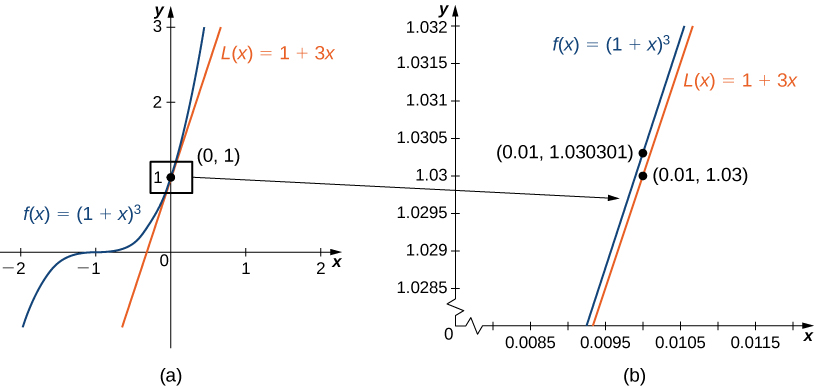
Linear approximations may be used in estimating roots and powers. In the next example, we find the linear approximation for $f(x)=(1+x)^n$ at $x=0$ , which can be used to estimate roots and powers for real numbers near 1. The same idea can be extended to a function of the form $f(x)=(m+x)^n$ to estimate roots and powers near a different number $m$ .

Example: Approximating Roots and Powers

Find the linear approximation of $f(x)=(1+x)^n$ at $x=0$ . Use this approximation to estimate $(1.01)^3$ .

Show Solution

The linear approximation at $x=0$ is given by

L (x) = f (0) + f^{'} (0) (x - 0)

$L(x)=f(0)+f^{\prime}(0)(x-0)$ .

Because

\begin{matrix} f (x) = (1 + x)^{n} & \Rightarrow & f (0) = 1 f^{'} (x) = n (1 + x)^{n - 1} & \Rightarrow & f^{'} (0) = n, \end{matrix}

$\begin{array}{lll} f(x)=(1+x)^n & \Rightarrow & f(0)=1 \\ f^{\prime}(x)=n(1+x)^{n-1} & \Rightarrow & f^{\prime}(0)=n, \end{array}$

the linear approximation is given by Figure 4a.

L (x) = 1 + n (x - 0) = 1 + n x

$L(x)=1+n(x-0)=1+nx$

We can approximate $(1.01)^3$ by evaluating $L(0.01)$ when $n=3$ . We conclude that

(1.01)^{3} = f (1.01) \approx L (1.01) = 1 + 3 (0.01) = 1.03

$(1.01)^3=f(1.01)\approx L(1.01)=1+3(0.01)=1.03$ .

This figure has two parts a and b. In figure a, the line f(x) = (1 + x)3 is shown with its tangent line at (0, 1). In figure b, the area near the tangent point is blown up to show how good of an approximation the tangent is near (0, 1).

Figure 4. (a) The linear approximation of $f(x)$ at $x=0$ is $L(x)$ . (b) The actual value of $1.01^3$ is 1.030301. The linear approximation of $f(x)$ at $x=0$ estimates $1.01^3$ to be 1.03.

Try It

Find the linear approximation of $f(x)=(1+x)^4$ at $x=0$ without using the result from the preceding example.

Hint

$f^{\prime}(x)=4(1+x)^3$

Show Solution

$L(x)=1+4x$

Module 4: Applications of Derivatives