End Behavior

Learning Outcomes

Estimate the end behavior of a function as 𝑥 increases or decreases without bound

Recognize an oblique asymptote on the graph of a function

The behavior of a function as $x\to \pm \infty$ is called the function’s end behavior. At each of the function’s ends, the function could exhibit one of the following types of behavior:

The function $f(x)$ approaches a horizontal asymptote $y=L$ .
The function $f(x)\to \infty$ or $f(x)\to −\infty$ .
The function does not approach a finite limit, nor does it approach $\infty$ or $−\infty$ . In this case, the function may have some oscillatory behavior.

Let’s consider several classes of functions here and look at the different types of end behaviors for these functions.

End Behavior for Polynomial Functions

Consider the power function $f(x)=x^n$ where $n$ is a positive integer. From Figure 11 and Figure 12, we see that

lim x \to \infty x^{n} = \infty; n = 1, 2, 3, \dots

$\underset{x\to \infty }{\lim}x^n=\infty; \, n=1,2,3, \cdots$

and

lim x \to - \infty x^{n} = {\begin{matrix} \infty; & n = 2, 4, 6, \dots - \infty; & n = 1, 3, 5, \dots \end{matrix}

$\underset{x\to −\infty }{\lim}x^n=\begin{cases} \infty; & n=2,4,6,\cdots \\ -\infty; & n=1,3,5,\cdots \end{cases}$

The functions x2, x4, and x6 are graphed, and it is apparent that as the exponent grows the functions increase more quickly.

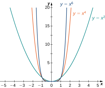
Figure 11. For power functions with an even power of $n$ , $\underset{x\to \infty }{\lim}x^n=\infty =\underset{x\to −\infty }{\lim}x^n$ .

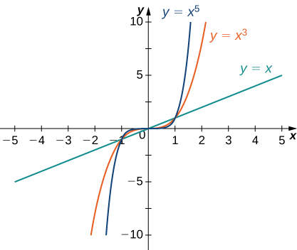
The functions x, x3, and x5 are graphed, and it is apparent that as the exponent grows the functions increase more quickly.

Figure 12. For power functions with an odd power of $n$ , $\underset{x\to \infty }{\lim}x^n=\infty$ and $\underset{x\to −\infty}{\lim}x^n=−\infty$ .

Using these facts, it is not difficult to evaluate $\underset{x\to \infty }{\lim}cx^n$ and $\underset{x\to −\infty }{\lim}cx^n$ , where $c$ is any constant and $n$ is a positive integer. If $c>0$ , the graph of $y=cx^n$ is a vertical stretch or compression of $y=x^n$ , and therefore

lim x \to \infty c x^{n} = lim x \to \infty x^{n}

$\underset{x\to \infty }{\lim}cx^n=\underset{x\to \infty }{\lim}x^n$ and

lim x \to - \infty c x^{n} = lim x \to - \infty x^{n}

$\underset{x\to −\infty }{\lim}cx^n=\underset{x\to −\infty}{\lim}x^n$ if

c > 0

$c>0$

If $c<0$ , the graph of $y=cx^n$ is a vertical stretch or compression combined with a reflection about the $x$ -axis, and therefore

lim x \to \infty c x^{n} = - lim x \to \infty x^{n}

$\underset{x\to \infty }{\lim}cx^n=−\underset{x\to \infty }{\lim}x^n$ and

lim x \to - \infty c x^{n} = - lim x \to - \infty x^{n}

$\underset{x\to −\infty}{\lim}cx^n=−\underset{x\to −\infty }{\lim}x^n$ if

c < 0

$c<0$

If $c=0, \, y=cx^n=0$ , in which case $\underset{x\to \infty }{\lim}cx^n=0=\underset{x\to −\infty }{\lim}cx^n$ .

Example: Limits at Infinity for Power Functions

For each function $f$ , evaluate $\underset{x\to \infty }{\lim}f(x)$ and $\underset{x\to −\infty }{\lim}f(x)$ .

$f(x)=-5x^3$
$f(x)=2x^4$

Show Solution

Since the coefficient of $x^3$ is -5, the graph of $f(x)=-5x^3$ involves a vertical stretch and reflection of the graph of $y=x^3$ about the $x$ -axis. Therefore, $\underset{x\to \infty }{\lim}(-5x^3)=−\infty$ and $\underset{x\to −\infty }{\lim}(-5x^3)=\infty$ .
Since the coefficient of $x^4$ is 2, the graph of $f(x)=2x^4$ is a vertical stretch of the graph of $y=x^4$ . Therefore, $\underset{x\to \infty }{\lim}2x^4=\infty$ and $\underset{x\to −\infty }{\lim}2x^4=\infty$ .

Watch the following video to see the worked solution to Example: Limits at Infinity for Power Functions.

Closed Captioning and Transcript Information for Video

Try It

Let $f(x)=-3x^4$ . Find $\underset{x\to \infty }{\lim}f(x)$ .

Hint

Show Solution

$−\infty$

We now look at how the limits at infinity for power functions can be used to determine $\underset{x\to \pm \infty }{\lim}f(x)$ for any polynomial function $f$ . Consider a polynomial function

f (x) = a_{n} x^{n} + a_{n - 1} x^{n - 1} + \dots + a_{1} x + a_{0}

$f(x)=a_n x^n + a_{n-1} x^{n-1} + \cdots + a_1 x + a_0$

of degree $n \ge 1$ so that $a_n \ne 0$ . Factoring, we see that

f (x) = a_{n} x^{n} (1 + \frac{a_{n - 1}}{a_{n}} \frac{1}{x} + \dots + \frac{a_{1}}{a_{n}} \frac{1}{x^{n - 1}} + \frac{a_{0}}{a_{n}} \frac{1}{x^{n}})

$f(x)=a_n x^n (1+\frac{a_{n-1}}{a_n}\frac{1}{x}+ \cdots + \frac{a_1}{a_n}\frac{1}{x^{n-1}} + \frac{a_0}{a_n}\frac{1}{x^n})$ .

As $x\to \pm \infty$ , all the terms inside the parentheses approach zero except the first term. We conclude that

lim x \to \pm \infty f (x) = lim x \to \pm \infty a_{n} x^{n}

$\underset{x\to \pm \infty }{\lim}f(x)=\underset{x\to \pm \infty }{\lim} a_n x^n$ .

For example, the function $f(x)=5x^3-3x^2+4$ behaves like $g(x)=5x^3$ as $x\to \pm \infty$ as shown in Figure 13 and Table 1.

Both functions f(x) = 5x3 – 3x2 + 4 and g(x) = 5x3 are plotted. Their behavior for large positive and large negative numbers converges.

Figure 13. The end behavior of a polynomial is determined by the behavior of the term with the largest exponent.

Table 1. A polynomial’s end behavior is determined by the term with the largest exponent.
$x$	10	100	1000
$f(x)=5x^3-3x^2+4$	4704	4,970,004	4,997,000,004
$g(x)=5x^3$	5000	5,000,000	5,000,000,000
$x$	-10	-100	-1000
$f(x)=5x^3-3x^2+4$	-5296	-5,029,996	-5,002,999,996
$g(x)=5x^3$	-5000	-5,000,000	-5,000,000,000

End Behavior for Algebraic Functions

The end behavior for rational functions and functions involving radicals is a little more complicated than for polynomials. In the example below, we show that the limits at infinity of a rational function $f(x)=\frac{p(x)}{q(x)}$ depend on the relationship between the degree of the numerator and the degree of the denominator. To evaluate the limits at infinity for a rational function, we divide the numerator and denominator by the highest power of $x$ appearing in the denominator. This determines which term in the overall expression dominates the behavior of the function at large values of $x$ .

Note that this is not your first encounter with horizontal asymptotes. It may be helpful to recall what you already know about them.

Recall: Horizontal Asymptotes of Rational Functions

The horizontal asymptote of a rational function can be determined by looking at the degrees of the numerator and denominator.

Case 1: Degree of numerator is less than degree of denominator: horizontal asymptote at $y=0$
Case 2: Degree of numerator is greater than degree of denominator by one: no horizontal asymptote; slant asymptote.
- If the degree of the numerator is greater than the degree of the denominator by more than one, the end behavior of the function’s graph will mimic that of the graph of the reduced ratio of leading terms.
Case 3: Degree of numerator is equal to degree of denominator: horizontal asymptote at ratio of leading coefficients.

Example: Determining End Behavior for Rational Functions

For each of the following functions, determine the limits as $x\to \infty$ and $x\to −\infty$ . Then, use this information to describe the end behavior of the function.

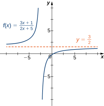
$f(x)=\frac{3x-1}{2x+5}$ (Note: The degree of the numerator and the denominator are the same.)
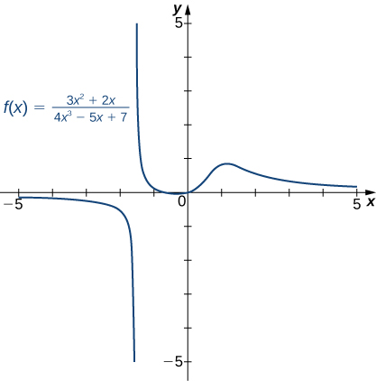
$f(x)=\frac{3x^2+2x}{4x^3-5x+7}$ (Note: The degree of numerator is less than the degree of the denominator.)
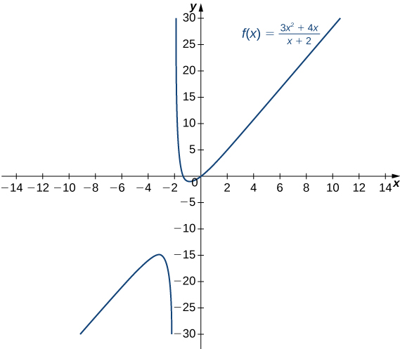
$f(x)=\frac{3x^2+4x}{x+2}$ (Note: The degree of numerator is greater than the degree of the denominator.)

Show Solution

The highest power of $x$ in the denominator is $x$ . Therefore, dividing the numerator and denominator by $x$ and applying the algebraic limit laws, we see that
$\begin{array}{ll} \underset{x\to \pm \infty }{\lim}\frac{3x-1}{2x+5} & =\underset{x\to \pm \infty }{\lim}\frac{3-1/x}{2+5/x} \\ & =\frac{\underset{x\to \pm \infty }{\lim}(3-1/x)}{\underset{x\to \pm \infty }{\lim}(2+5/x)} \\ & =\frac{\underset{x\to \pm \infty }{\lim}3-\underset{x\to \pm \infty }{\lim}1/x}{\underset{x\to \pm \infty }{\lim}2+\underset{x\to \pm \infty }{\lim}5/x} \\ & =\frac{3-0}{2+0}=\frac{3}{2}. \end{array}$

Since $\underset{x\to \pm \infty }{\lim}f(x)=\frac{3}{2}$ , we know that $y=\frac{3}{2}$ is a horizontal asymptote for this function as shown in the following graph.

Figure 14. The graph of this rational function approaches a horizontal asymptote as $x\to \pm \infty$ .
Since the largest power of $x$ appearing in the denominator is $x^3$ , divide the numerator and denominator by $x^3$ . After doing so and applying algebraic limit laws, we obtain
$\underset{x\to \pm \infty }{\lim}\frac{3x^2+2x}{4x^3-5x+7}=\underset{x\to \pm \infty }{\lim}\frac{3/x+2/x^2}{4-5/x^2+7/x^3}=\frac{3(0)+2(0)}{4-5(0)+7(0)}=0$

Therefore $f$ has a horizontal asymptote of $y=0$ as shown in the following graph.

Figure 15. The graph of this rational function approaches the horizontal asymptote $y=0$ as $x\to \pm \infty$ .
Dividing the numerator and denominator by $x$ , we have
$\underset{x\to \pm \infty }{\lim}\frac{3x^2+4x}{x+2}=\underset{x\to \pm \infty }{\lim}\frac{3x+4}{1+2/x}$ .

As $x\to \pm \infty$ , the denominator approaches 1. As $x\to \infty$ , the numerator approaches $+\infty$ . As $x\to −\infty$ , the numerator approaches $−\infty$ . Therefore $\underset{x\to \infty }{\lim}f(x)=\infty$ , whereas $\underset{x\to −\infty }{\lim}f(x)=−\infty$ as shown in the following figure.

Figure 16. As $x\to \infty$ , the values $f(x)\to \infty$ . As $x\to −\infty$ , the values $f(x)\to −\infty$ .

Watch the following video to see the worked solution to Example: Determining End Behavior for Rational Functions.

Closed Captioning and Transcript Information for Video

Try It

Evaluate $\underset{x\to \pm \infty }{\lim}\dfrac{3x^2+2x-1}{5x^2-4x+7}$ and use these limits to determine the end behavior of $f(x)=\dfrac{3x^2+2x-1}{5x^2-4x+7}$ .

Hint

Divide the numerator and denominator by $x^2$ .

Show Solution

$\frac{3}{5}$

Before proceeding, consider the graph of $f(x)=\frac{(3x^2+4x)}{(x+2)}$ shown in Figure 17. As $x\to \infty$ and $x\to −\infty$ , the graph of $f$ appears almost linear. Although $f$ is certainly not a linear function, we now investigate why the graph of $f$ seems to be approaching a linear function. First, using long division of polynomials, we can write

f (x) = \frac{3 x^{2} + 4 x}{x + 2} = 3 x - 2 + \frac{4}{x + 2}

$f(x)=\frac{3x^2+4x}{x+2}=3x-2+\frac{4}{x+2}$

Since $\frac{4}{(x+2)}\to 0$ as $x\to \pm \infty$ , we conclude that

lim x \to \pm \infty (f (x) - (3 x - 2)) = lim x \to \pm \infty \frac{4}{x + 2} = 0

$\underset{x\to \pm \infty }{\lim}(f(x)-(3x-2))=\underset{x\to \pm \infty }{\lim}\frac{4}{x+2}=0$

Therefore, the graph of $f$ approaches the line $y=3x-2$ as $x\to \pm \infty$ . This line is known as an oblique asymptote for $f$ (Figure 17).

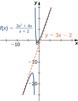
The function f(x) = (3x2 + 4x)/(x + 2) is plotted as is its diagonal asymptote y = 3x – 2.

Figure 17. The graph of the rational function $f(x)=(3x^2+4x)/(x+2)$ approaches the oblique asymptote $y=3x-2$ as $x\to \pm \infty$ .

We can summarize the results of the example above to make the following conclusion regarding end behavior for rational functions. Consider a rational function

f (x) = \frac{p (x)}{q (x)} = \frac{a_{n} x^{n} + a_{n - 1} x^{n - 1} + \dots + a_{1} x + a_{0}}{b_{m} x^{m} + b_{m - 1} x^{m - 1} + \dots + b_{1} x + b_{0}}

$f(x)=\frac{p(x)}{q(x)}=\frac{a_n x^n + a_{n-1} x^{n-1} + \cdots + a_1 x + a_0}{b_m x^m + b_{m-1} x^{m-1} + \cdots + b_1 x + b_0}$ ,

where $a_n\ne 0$ and $b_m \ne 0$ .

If the degree of the numerator is the same as the degree of the denominator $(n=m)$ , then $f$ has a horizontal asymptote of $y=a_n/b_m$ as $x\to \pm \infty$ .
If the degree of the numerator is less than the degree of the denominator [latex](n
If the degree of the numerator is greater than the degree of the denominator $(n>m)$ , then $f$ does not have a horizontal asymptote. The limits at infinity are either positive or negative infinity, depending on the signs of the leading terms. In addition, using long division, the function can be rewritten as
$f(x)=\frac{p(x)}{q(x)}=g(x)+\frac{r(x)}{q(x)}$ ,

where the degree of $r(x)$ is less than the degree of $q(x)$ . As a result, $\underset{x\to \pm \infty }{\lim}r(x)/q(x)=0$ . Therefore, the values of $[f(x)-g(x)]$ approach zero as $x\to \pm \infty$ . If the degree of $p(x)$ is exactly one more than the degree of $q(x)$ $(n=m+1)$ , the function $g(x)$ is a linear function. In this case, we call $g(x)$ an oblique asymptote.
Now let’s consider the end behavior for functions involving a radical.

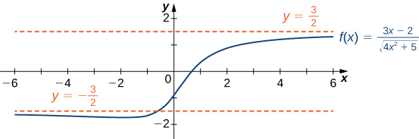
Example: Determining End Behavior for a Function Involving a Radical

Find the limits as $x\to \infty$ and $x\to −\infty$ for $f(x)=\frac{3x-2}{\sqrt{4x^2+5}}$ and describe the end behavior of $f$ .

Show Solution

Let’s use the same strategy as we did for rational functions: divide the numerator and denominator by a power of $x$ . To determine the appropriate power of $x$ , consider the expression $\sqrt{4x^2+5}$ in the denominator. Since

\sqrt{4 x^{2} + 5} \approx \sqrt{4 x^{2}} = 2 | x |

$\sqrt{4x^2+5}\approx \sqrt{4x^2}=2|x|$

for large values of $x$ in effect $x$ appears just to the first power in the denominator. Therefore, we divide the numerator and denominator by $|x|$ . Then, using the fact that $|x|=x$ for $x>0$ , $|x|=−x$ for $x<0$ , and $|x|=\sqrt{x^2}$ for all $x$ , we calculate the limits as follows:

\begin{matrix} lim x \to \infty \frac{3 x - 2}{\sqrt{4 x^{2} + 5}} & = & lim x \to \infty \frac{(1 / | x |) (3 x - 2)}{(1 / | x |) \sqrt{4 x^{2} + 5}} = & lim x \to \infty \frac{(1 / x) (3 x - 2)}{\sqrt{(1 / x^{2}) (4 x^{2} + 5)}} = & lim x \to \infty \frac{3 - 2 / x}{\sqrt{4 + 5 / x^{2}}} = \frac{3}{\sqrt{4}} = \frac{3}{2} lim x \to - \infty \frac{3 x - 2}{\sqrt{4 x^{2} + 5}} & = & lim x \to - \infty \frac{(1 / | x |) (3 x - 2)}{(1 / | x |) \sqrt{4 x^{2} + 5}} = & lim x \to - \infty \frac{(- 1 / x) (3 x - 2)}{\sqrt{(1 / x^{2}) (4 x^{2} + 5)}} = & lim x \to - \infty \frac{- 3 + 2 / x}{\sqrt{4 + 5 / x^{2}}} = \frac{- 3}{\sqrt{4}} = \frac{- 3}{2} . \end{matrix}

$\begin{array}{lll} \underset{x\to \infty }{\lim}\frac{3x-2}{\sqrt{4x^2+5}} & = & \underset{x\to \infty }{\lim}\frac{(1/|x|)(3x-2)}{(1/|x|)\sqrt{4x^2+5}} \\ & = & \underset{x\to \infty }{\lim}\frac{(1/x)(3x-2)}{\sqrt{(1/x^2)(4x^2+5)}} \\ & = & \underset{x\to \infty }{\lim}\frac{3-2/x}{\sqrt{4+5/x^2}}=\frac{3}{\sqrt{4}}=\frac{3}{2} \\ \underset{x\to −\infty }{\lim}\frac{3x-2}{\sqrt{4x^2+5}} & = & \underset{x\to −\infty }{\lim}\frac{(1/|x|)(3x-2)}{(1/|x|)\sqrt{4x^2+5}} \\ & = & \underset{x\to −\infty }{\lim}\frac{(-1/x)(3x-2)}{\sqrt{(1/x^2)(4x^2+5)}} \\ & = & \underset{x\to −\infty }{\lim}\frac{-3+2/x}{\sqrt{4+5/x^2}}=\frac{-3}{\sqrt{4}}=\frac{-3}{2}. \end{array}$

Therefore, $f(x)$ approaches the horizontal asymptote $y=\frac{3}{2}$ as $x\to \infty$ and the horizontal asymptote $y=-\frac{3}{2}$ as $x\to −\infty$ as shown in the following graph.

The function f(x) = (3x − 2)/(the square root of the quantity (4x2 + 5)) is plotted. It has two horizontal asymptotes at y = ±3/2, and it crosses y = −3/2 before converging toward it from below.

Figure 18. This function has two horizontal asymptotes and it crosses one of the asymptotes.

Try It

Evaluate $\underset{x\to \infty }{\lim}\frac{\sqrt{3x^2+4}}{x+6}$ .

Hint

Divide the numerator and denominator by $|x|$ .

Show Solution

$\pm \sqrt{3}$

Try It

Determining End Behavior for Transcendental Functions

The six basic trigonometric functions are periodic and do not approach a finite limit as $x\to \pm \infty$ . For example, $\sin x$ oscillates between 1 and -1 (Figure 19). The tangent function $x$ has an infinite number of vertical asymptotes as $x\to \pm \infty$ ; therefore, it does not approach a finite limit nor does it approach $\pm \infty$ as $x\to \pm \infty$ as shown in (Figure 20).

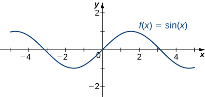
Figure 19. The function $f(x)= \sin x$ oscillates between 1 and -1 as $x\to \pm \infty$

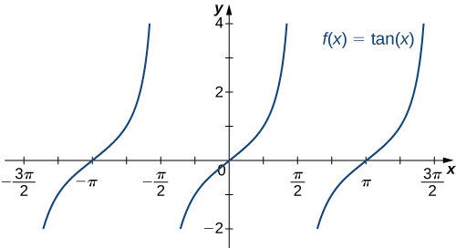
Figure 20. The function $f(x)= \tan x$ does not approach a limit and does not approach $\pm \infty$ as $x\to \pm \infty$

Recall that for any base $b>0, \, b\ne 1$ , the function $y=b^x$ is an exponential function with domain $(−\infty ,\infty )$ and range $(0,\infty )$ . If $b>1, \, y=b^x$ is increasing over $(−\infty ,\infty )$ . If [latex]01[/latex]. Therefore, $f(x)=e^x$ is increasing on $(−\infty ,\infty )$ and the range is $(0,\infty)$ . The exponential function $f(x)=e^x$ approaches $\infty$ as $x\to \infty$ and approaches 0 as $x\to −\infty$ as shown in (Figure) and (Figure).

End behavior of the natural exponential function
$x$	-5	-2	0	2	5
$e^x$	0.00674	0.135	1	7.389	148.413

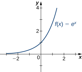
Figure 21. The exponential function approaches zero as $x\to −\infty$ and approaches $\infty$ as $x\to \infty$ .

Recall that the natural logarithm function $f(x)=\ln (x)$ is the inverse of the natural exponential function $y=e^x$ . Therefore, the domain of $f(x)=\ln (x)$ is $(0,\infty )$ and the range is $(−\infty ,\infty )$ . The graph of $f(x)=\ln (x)$ is the reflection of the graph of $y=e^x$ about the line $y=x$ . Therefore, $\ln (x)\to −\infty$ as $x\to 0^+$ and $\ln (x)\to \infty$ as $x\to \infty$ as shown in (Figure) and (Figure).

End behavior of the natural logarithm function
$x$	0.01	0.1	1	10	100
$\ln (x)$	-4.605	-2.303	0	2.303	4.605

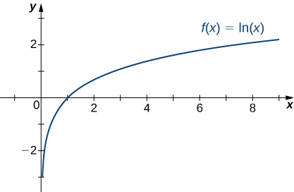
Figure 22. The natural logarithm function approaches $\infty$ as $x\to \infty$ .

example: Determining End Behavior for a Transcendental Function

Find the limits as $x\to \infty$ and $x\to −\infty$ for $f(x)=\frac{(2+3e^x)}{(7-5e^x)}$ and describe the end behavior of $f$ .

Show Solution

To find the limit as $x\to \infty$ , divide the numerator and denominator by $e^x$ :

$\begin{array}{ll} \underset{x\to \infty }{\lim}f(x) & =\underset{x\to \infty }{\lim}\frac{2+3e^x}{7-5e^x} \\ & =\underset{x\to \infty }{\lim}\frac{(2/e^x)+3}{(7/e^x)-5}. \end{array}$

As shown in Figure 21, $e^x\to \infty$ as $x\to \infty$ . Therefore,

$\underset{x\to \infty }{\lim}\frac{2}{e^x}=0=\underset{x\to \infty }{\lim}\frac{7}{e^x}$ .

We conclude that $\underset{x\to \infty }{\lim}f(x)=-\frac{3}{5}$ , and the graph of $f$ approaches the horizontal asymptote $y=-\frac{3}{5}$ as $x\to \infty$ . To find the limit as $x\to −\infty$ , use the fact that $e^x \to 0$ as $x\to −\infty$ to conclude that $\underset{x\to -\infty }{\lim}f(x)=\frac{2}{7}$ , and therefore the graph of approaches the horizontal asymptote $y=\frac{2}{7}$ as $x\to −\infty$ .

Watch the following video to see the worked solution to Example: Determining End Behavior for a Transcendental Function.

Closed Captioning and Transcript Information for Video

Try It

Find the limits as $x\to \infty$ and $x\to −\infty$ for $f(x)=\dfrac{(3e^x-4)}{(5e^x+2)}$ .

Hint

$\underset{x\to \infty }{\lim}e^x=\infty$ and $\underset{x\to -\infty }{\lim}e^x=0$ .

Show Solution

$\underset{x\to \infty }{\lim}f(x)=\frac{3}{5}$ , $\underset{x\to −\infty }{\lim}f(x)=-2$

Module 4: Applications of Derivatives

Learning Outcomes

End Behavior for Polynomial Functions

Example: Limits at Infinity for Power Functions

Try It

End Behavior for Algebraic Functions

Recall: Horizontal Asymptotes of Rational Functions

Example: Determining End Behavior for Rational Functions

Try It

Example: Determining End Behavior for a Function Involving a Radical

Try It

Try It

Determining End Behavior for Transcendental Functions

example: Determining End Behavior for a Transcendental Function

Try It

Candela Citations