Learning Outcomes
- Identify the form of an exponential function
- Explain the difference between the graphs of [latex]x^b[/latex] and [latex]b^x[/latex]
- Recognize the significance of the number [latex]e[/latex]
Exponential functions arise in many applications. One common example is population growth.
For example, if a population starts with [latex]P_0[/latex] individuals and then grows at an annual rate of [latex]2\%[/latex], its population after 1 year is
Its population after 2 years is
In general, its population after [latex]t[/latex] years is
which is an exponential function. More generally, any function of the form [latex]f(x)=b^x[/latex], where [latex]b>0, \, b \ne 1[/latex], is an exponential function with base [latex]b[/latex] and exponent [latex]x[/latex]. Exponential functions have constant bases and variable exponents. Note that a function of the form [latex]f(x)=x^b[/latex] for some constant [latex]b[/latex] is not an exponential function but a power function.
To see the difference between an exponential function and a power function, we compare the functions [latex]y=x^2[/latex] and [latex]y=2^x[/latex]. In the table below, we see that both [latex]2^x[/latex] and [latex]x^2[/latex] approach infinity as [latex]x \to \infty[/latex]. Eventually, however, [latex]2^x[/latex] becomes larger than [latex]x^2[/latex] and grows more rapidly as [latex]x \to \infty[/latex]. In the opposite direction, as [latex]x \to −\infty, \, x^2 \to \infty[/latex], whereas [latex]2^x \to 0[/latex]. The line [latex]y=0[/latex] is a horizontal asymptote for [latex]y=2^x[/latex].
| [latex]\mathbf{x}[/latex] | -3 | -2 | -1 | 0 | 1 | 2 | 3 | 4 | 5 | 6 |
| [latex]\mathbf{x^2}[/latex] | 9 | 4 | 1 | 0 | 1 | 4 | 9 | 16 | 25 | 36 |
| [latex]\mathbf{2^x}[/latex] | [latex]1/8[/latex] | [latex]1/4[/latex] | [latex]1/2[/latex] | 1 | 2 | 4 | 8 | 16 | 32 | 64 |
In Figure 1, we graph both [latex]y=x^2[/latex] and [latex]y=2^x[/latex] to show how the graphs differ.
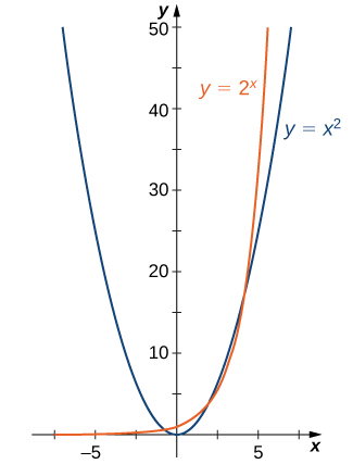
Figure 1. Both [latex]2^x[/latex] and [latex]x^2[/latex] approach infinity as [latex]x \to \infty[/latex], but [latex]2^x[/latex] grows more rapidly than [latex]x^2[/latex]. As [latex]x \to −\infty, \, x^2 \to \infty[/latex], whereas [latex]2^x \to 0[/latex].
Evaluating Exponential Functions
Recall the properties of exponents: If [latex]x[/latex] is a positive integer, then we define [latex]b^x=b·b \cdots b[/latex] (with [latex]x[/latex] factors of [latex]b[/latex]). If [latex]x[/latex] is a negative integer, then [latex]x=−y[/latex] for some positive integer [latex]y[/latex], and we define [latex]b^x=b^{−y}=1/b^y[/latex]. Also, [latex]b^0[/latex] is defined to be 1. If [latex]x[/latex] is a rational number, then [latex]x=p/q[/latex], where [latex]p[/latex] and [latex]q[/latex] are integers and [latex]b^x=b^{p/q}=\sqrt[q]{b^p}[/latex]. For example, [latex]9^{3/2}=\sqrt{9^3}=27[/latex]. However, how is [latex]b^x[/latex] defined if [latex]x[/latex] is an irrational number? For example, what do we mean by [latex]2^{\sqrt{2}}[/latex]? This is too complex a question for us to answer fully right now; however, we can make an approximation. In the table below, we list some rational numbers approaching [latex]\sqrt{2}[/latex], and the values of [latex]2^x[/latex] for each rational number [latex]x[/latex] are presented as well. We claim that if we choose rational numbers [latex]x[/latex] getting closer and closer to [latex]\sqrt{2}[/latex], the values of [latex]2^x[/latex] get closer and closer to some number [latex]L[/latex]. We define that number [latex]L[/latex] to be [latex]2^{\sqrt{2}}[/latex].
| [latex]\mathbf{x}[/latex] | 1.4 | 1.41 | 1.414 | 1.4142 | 1.41421 | 1.414213 |
| [latex]\mathbf{2^x}[/latex] | 2.639 | 2.65737 | 2.66475 | 2.665119 | 2.665138 | 2.665143 |
Example: Bacterial Growth
Suppose a particular population of bacteria is known to double in size every 4 hours. If a culture starts with 1000 bacteria, the number of bacteria after 4 hours is [latex]n(4)=1000·2[/latex]. The number of bacteria after 8 hours is [latex]n(8)=n(4)·2=1000·2^2[/latex]. In general, the number of bacteria after [latex]4m[/latex] hours is [latex]n(4m)=1000·2^m[/latex]. Letting [latex]t=4m[/latex], we see that the number of bacteria after [latex]t[/latex] hours is [latex]n(t)=1000·2^{t/4}[/latex]. Find the number of bacteria after 6 hours, 10 hours, and 24 hours.
Try It
Given the exponential function [latex]f(x)=100·3^{x/2}[/latex], evaluate [latex]f(4)[/latex] and [latex]f(10)[/latex].
Try It
Graphing Exponential Functions
It may be helpful to recall arrow and interval notation before you explore this section.
Recall: Arrow and interval notation
| Arrow Notation | |
|---|---|
| Symbol | Meaning |
| [latex]x\to \infty[/latex] | [latex]x[/latex] approaches infinity ([latex]x[/latex] increases without bound) |
| [latex]x\to -\infty[/latex] | [latex]x[/latex] approaches negative infinity ([latex]x[/latex] decreases without bound) |
| [latex]f\left(x\right)\to \infty[/latex] | the output approaches infinity (the output increases without bound) |
| [latex]f\left(x\right)\to -\infty[/latex] | the output approaches negative infinity (the output decreases without bound) |
| [latex]f\left(x\right)\to a[/latex] | the output approaches [latex]a[/latex] |
| Inequality Notation | Set-builder Notation | Interval Notation | |
|---|---|---|---|
 |
[latex]5| [latex]\{h | 5 < h \le 10\}[/latex] |
[latex](5,10][/latex] |
|
 |
[latex]5\le h<10[/latex] | [latex]\{h | 5 \le h < 10\}[/latex] | [latex][5,10)[/latex] |
 |
[latex]5| [latex]\{h | 5 < h < 10\}[/latex] |
[latex](5,10)[/latex] |
|
 |
[latex]h<10[/latex] | [latex]\{h | h < 10\}[/latex] | [latex](-\infty,10)[/latex] |
 |
[latex]h>10[/latex] | [latex]\{h | h > 10\}[/latex] | [latex](10,\infty)[/latex] |
 |
All real numbers | [latex]\mathbf{R}[/latex] | [latex](−\infty,\infty)[/latex] |
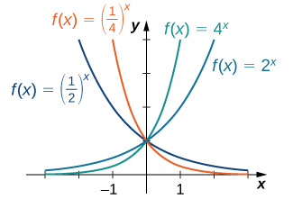
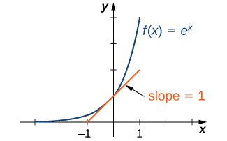
For any base [latex]b>0, \, b\ne 1[/latex], the exponential function [latex]f(x)=b^x[/latex] is defined for all real numbers [latex]x[/latex] and [latex]b^x>0[/latex]. Therefore, the domain of [latex]f(x)=b^x[/latex] is [latex](−\infty ,\infty)[/latex] and the range is [latex](0,\infty)[/latex]. To graph [latex]b^x[/latex], we note that for [latex]b>1, \, b^x[/latex] is increasing on [latex](−\infty ,\infty)[/latex] and [latex]b^x \to \infty[/latex] as [latex]x \to \infty[/latex], whereas [latex]b^x \to 0[/latex] as [latex]x \to −\infty[/latex]. On the other hand, if [latex]0 Figure 2. If [latex]b>1[/latex], then [latex]b^x[/latex] is increasing on [latex](−\infty ,\infty)[/latex]. If [latex]0<b<1[/latex], then [latex]b^x[/latex] is decreasing on [latex](−\infty ,\infty)[/latex]. Note that exponential functions satisfy the general laws of exponents. To remind you of these laws, we state them as rules. For any constants [latex]a>0, \, b>0[/latex], and for all [latex]x[/latex] and [latex]y[/latex], Use the laws of exponents to simplify each of the following expressions. Watch the following video to see the worked solution to Example: Using the Laws of Exponents Use the laws of exponents to simplify [latex]\dfrac{(6x^{-3}y^2)}{(12x^{-4}y^5)}[/latex]. A special type of exponential function appears frequently in real-world applications. To describe it, consider the following example of exponential growth, which arises from compounding interest in a savings account. Suppose a person invests [latex]P[/latex] dollars in a savings account with an annual interest rate [latex]r[/latex], compounded annually. The amount of money after 1 year is The amount of money after 2 years is More generally, the amount after [latex]t[/latex] years is If the money is compounded 2 times per year, the amount of money after half a year is The amount of money after 1 year is After [latex]t[/latex] years, the amount of money in the account is More generally, if the money is compounded [latex]n[/latex] times per year, the amount of money in the account after [latex]t[/latex] years is given by the function What happens as [latex]n\to \infty[/latex]? To answer this question, we let [latex]m=n/r[/latex] and write and examine the behavior of [latex](1+\frac{1}{m})^m[/latex] as [latex]m\to \infty[/latex], using a table of values. Looking at this table, it appears that [latex](1+\frac{1}{m})^m[/latex] is approaching a number between 2.7 and 2.8 as [latex]m\to \infty[/latex]. In fact, [latex](1+\frac{1}{m})^m[/latex] does approach some number as [latex]m\to \infty[/latex]. We call this number [latex]e[/latex]. To six decimal places of accuracy, The letter [latex]e[/latex] was first used to represent this number by the Swiss mathematician Leonhard Euler during the 1720s. Although Euler did not discover the number, he showed many important connections between [latex]e[/latex] and logarithmic functions. We still use the notation [latex]e[/latex] today to honor Euler’s work because it appears in many areas of mathematics and because we can use it in many practical applications. Returning to our savings account example, we can conclude that if a person puts [latex]P[/latex] dollars in an account at an annual interest rate [latex]r[/latex], compounded continuously, then [latex]A(t)=Pe^{rt}[/latex]. This function may be familiar. Since functions involving base [latex]e[/latex] arise often in applications, we call the function [latex]f(x)=e^x[/latex] the natural exponential function. Not only is this function interesting because of the definition of the number [latex]e[/latex], but also, as discussed next, its graph has an important property. Since [latex]e>1[/latex], we know [latex]e^x[/latex] is increasing on [latex](−\infty ,\infty)[/latex]. In Figure 3, we show a graph of [latex]f(x)=e^x[/latex] along with a tangent line to the graph of at [latex]x=0[/latex]. We give a precise definition of tangent line in the next module; but, informally, we say a tangent line to a graph of [latex]f[/latex] at [latex]x=a[/latex] is a line that passes through the point [latex](a,f(a))[/latex] and has the same “slope” as [latex]f[/latex] at that point. The function [latex]f(x)=e^x[/latex] is the only exponential function [latex]b^x[/latex] with tangent line at [latex]x=0[/latex] that has a slope of 1. As we see later in the text, having this property makes the natural exponential function the simplest exponential function to use in many instances. Figure 3. The graph of [latex]f(x)=e^x[/latex] has a tangent line with slope 1 at [latex]x=0[/latex]. Suppose [latex]\$500[/latex] is invested in an account at an annual interest rate of [latex]r=5.5\%[/latex], compounded continuously. Watch the following video to see the worked solution to Example: Compounding Interest If [latex]\$750[/latex] is invested in an account at an annual interest rate of [latex]4\%[/latex], compounded continuously, find a formula for the amount of money in the account after [latex]t[/latex] years. Find the amount of money after 30 years.
Laws of Exponents
Example: Using the Laws of Exponents
Try It
Try It
The Number [latex]e[/latex]
[latex]\mathbf{m}[/latex]
10
100
1000
10,000
100,000
1,000,000
[latex]\mathbf{(1+\frac{1}{m})^m}[/latex]
2.5937
2.7048
2.71692
2.71815
2.718268
2.718280
Example: Compounding Interest
Try It
Try It
Candela Citations
