Learning Outcomes
- Identify the form of a logarithmic function
- Explain the relationship between exponential and logarithmic functions
- Describe how to calculate a logarithm to a different base
Using our understanding of exponential functions, we can discuss their inverses, which are the logarithmic functions. Recall the definition of an inverse function.
Recall: Inverse Function
For any one-to-one function [latex]f\left(x\right)=y[/latex], a function [latex]{f}^{-1}\left(x\right)[/latex] is an inverse function of [latex]f[/latex] if [latex]{f}^{-1}\left(y\right)=x[/latex]. This can also be written as [latex]{f}^{-1}\left(f\left(x\right)\right)=x[/latex] for all [latex]x[/latex] in the domain of [latex]f[/latex]. It also follows that [latex]f\left({f}^{-1}\left(x\right)\right)=x[/latex] for all [latex]x[/latex] in the domain of [latex]{f}^{-1}[/latex] if [latex]{f}^{-1}[/latex] is the inverse of [latex]f[/latex].
The notation [latex]{f}^{-1}[/latex] is read “[latex]f[/latex] inverse.” Like any other function, we can use any variable name as the input for [latex]{f}^{-1}[/latex], so we will often write [latex]{f}^{-1}\left(x\right)[/latex], which we read as [latex]"f[/latex] inverse of [latex]x[/latex]“.
Logarithmic functions come in handy when we need to consider any phenomenon that varies over a wide range of values, such as pH in chemistry or decibels in sound levels.
The exponential function [latex]f(x)=b^x[/latex] is one-to-one, with domain [latex](−\infty ,\infty)[/latex] and range [latex](0,\infty )[/latex]. Therefore, it has an inverse function, called the logarithmic function with base [latex]b[/latex]. For any [latex]b>0, \, b \ne 1[/latex], the logarithmic function with base [latex]b[/latex], denoted [latex]\log_b[/latex], has domain [latex](0,\infty )[/latex] and range [latex](−\infty ,\infty )[/latex], and satisfies
For example,
Furthermore, since [latex]y=\log_b (x)[/latex] and [latex]y=b^x[/latex] are inverse functions,
The most commonly used logarithmic function is the function [latex]\log_e (x)[/latex]. Since this function uses natural [latex]e[/latex] as its base, it is called the natural logarithm. Here we use the notation [latex]\ln(x)[/latex] or [latex]\ln x[/latex] to mean [latex]\log_e (x)[/latex]. For example,
Since the functions [latex]f(x)=e^x[/latex] and [latex]g(x)=\ln(x)[/latex] are inverses of each other,
and their graphs are symmetric about the line [latex]y=x[/latex] (Figure 4).
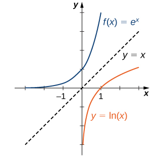
Figure 4: The functions [latex]y=e^x[/latex] and [latex]y=\ln(x)[/latex] are inverses of each other, so their graphs are symmetric about the line [latex]y=x[/latex].
In general, for any base [latex]b>0, \, b\ne 1[/latex], the function [latex]g(x)=\log_b (x)[/latex] is symmetric about the line [latex]y=x[/latex] with the function [latex]f(x)=b^x[/latex]. Using this fact and the graphs of the exponential functions, we graph functions [latex]\log_b (x)[/latex] for several values of [latex]b>1[/latex] (Figure 5).
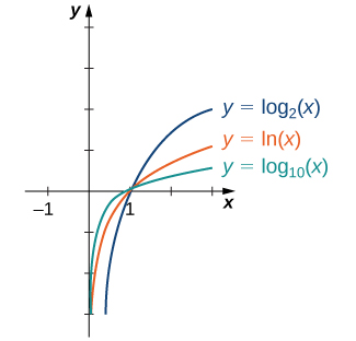
Figure 5: Graphs of [latex]y=\log_b (x)[/latex] are depicted for [latex]b=2, \, e, \, 10[/latex].
Before solving some equations involving exponential and logarithmic functions, let’s review the basic properties of logarithms.
Properties of Logarithms
If [latex]a,b,c>0, \, b\ne 1[/latex], and [latex]r[/latex] is any real number, then
[latex]\begin{array}{cccc}1.\phantom{\rule{2em}{0ex}}\log_b (ac)=\log_b (a)+\log_b (c)\hfill & & & \text{(Product property)}\hfill \\ 2.\phantom{\rule{2em}{0ex}}\log_b(\frac{a}{c})=\log_b (a) -\log_b (c)\hfill & & & \text{(Quotient property)}\hfill \\ 3.\phantom{\rule{2em}{0ex}}\log_b (a^r)=r \log_b (a)\hfill & & & \text{(Power property)}\hfill \end{array}[/latex]
Example: Solving Equations Involving Exponential Functions
Solve each of the following equations for [latex]x[/latex].
- [latex]5^x=2[/latex]
- [latex]e^x+6e^{−x}=5[/latex]
Watch the following video to see the worked solution to Example: Solving Equations Involving Exponential Functions
Try It
Solve [latex]\dfrac{e^{2x}}{(3+e^{2x})}=\dfrac{1}{2}[/latex].
Example: Solving Equations Involving Logarithmic Functions
Solve each of the following equations for [latex]x[/latex].
- [latex]\ln \left(\frac{1}{x}\right)=4[/latex]
- [latex]\log_{10} \sqrt{x}+ \log_{10} x=2[/latex]
- [latex]\ln(2x)-3 \ln(x^2)=0[/latex]
Watch the following video to see the worked solution to Example: Solving Equations Involving Logarithmic Functions
Try It
Solve [latex]\ln(x^3)-4 \ln (x)=1[/latex].
Try It
When evaluating a logarithmic function with a calculator, you may have noticed that the only options are [latex]\log_{10}[/latex] or log, called the common logarithm, or ln, which is the natural logarithm. However, exponential functions and logarithm functions can be expressed in terms of any desired base [latex]b[/latex]. If you need to use a calculator to evaluate an expression with a different base, you can apply the change-of-base formulas first. Using this change of base, we typically write a given exponential or logarithmic function in terms of the natural exponential and natural logarithmic functions.
Try It
Change-of-Base Formulas
Let [latex]a>0, \, b>0[/latex], and [latex]a\ne 1, \, b\ne 1[/latex].
- [latex]a^x=b^{x \log_b a}[/latex] for any real number [latex]x[/latex].
If [latex]b=e[/latex], this equation reduces to [latex]a^x=e^{x \log_e a}=e^{x \ln a}[/latex]. - [latex]\log_a x=\frac{\log_b x}{\log_b a}[/latex] for any real number [latex]x>0[/latex].
If [latex]b=e[/latex], this equation reduces to [latex]\log_a x=\frac{\ln x}{\ln a}[/latex].
Proof
For the first change-of-base formula, we begin by making use of the power property of logarithmic functions. We know that for any base [latex]b>0, \, b\ne 1, \, \log_b (a^x)=x \log_b a[/latex]. Therefore,
In addition, we know that [latex]b^x[/latex] and [latex]\log_b (x)[/latex] are inverse functions. Therefore,
Combining these last two equalities, we conclude that [latex]a^x=b^{x \log_b a}[/latex].
To prove the second property, we show that
Let [latex]u=\log_b a, \, v=\log_a x[/latex], and [latex]w=\log_b x[/latex]. We will show that [latex]u·v=w[/latex]. By the definition of logarithmic functions, we know that [latex]b^u=a, \, a^v=x[/latex], and [latex]b^w=x[/latex]. From the previous equations, we see that
Therefore, [latex]b^{uv}=b^w[/latex]. Since exponential functions are one-to-one, we can conclude that [latex]u·v=w[/latex].
[latex]_\blacksquare[/latex]
Example: Changing Bases
Use a calculating utility to evaluate [latex]\log_3 7[/latex] with the change-of-base formula presented earlier.
Try It
Use the change-of-base formula and a calculating utility to evaluate [latex]\log_4 6[/latex].
Try It
Compare the relative severity of a magnitude 8.4 earthquake with a magnitude 7.4 earthquake.
Try It
Candela Citations
- 1.5 Exponential and Logarithmic Functions. Authored by: Ryan Melton. License: CC BY: Attribution
- Calculus Volume 1. Authored by: Gilbert Strang, Edwin (Jed) Herman. Provided by: OpenStax. Located at: https://openstax.org/details/books/calculus-volume-1. License: CC BY-NC-SA: Attribution-NonCommercial-ShareAlike. License Terms: Access for free at https://openstax.org/books/calculus-volume-1/pages/1-introduction
