Learning Outcomes
- Identify the hyperbolic functions, their graphs, and basic identities
The hyperbolic functions are defined in terms of certain combinations of [latex]e^x[/latex] and [latex]e^{−x}[/latex]. These functions arise naturally in various engineering and physics applications, including the study of water waves and vibrations of elastic membranes. Another common use for a hyperbolic function is the representation of a hanging chain or cable, also known as a catenary. If we introduce a coordinate system so that the low point of the chain lies along the [latex]y[/latex]-axis, we can describe the height of the chain in terms of a hyperbolic function. First, we define the hyperbolic functions.
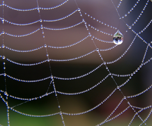
Figure 6. The shape of a strand of silk in a spider’s web can be described in terms of a hyperbolic function. The same shape applies to a chain or cable hanging from two supports with only its own weight. (credit: “Mtpaley”, Wikimedia Commons)
Definition
Hyperbolic cosine
Hyperbolic sine
Hyperbolic tangent
Hyperbolic cosecant
Hyperbolic secant
Hyperbolic cotangent
The name cosh rhymes with “gosh,” whereas the name sinh is pronounced “cinch.” Tanh, sech, csch, and coth are pronounced “tanch,” “seech,” “coseech,” and “cotanch,” respectively.
Using the definition of [latex]\cosh(x)[/latex] and principles of physics, it can be shown that the height of a hanging chain, such as the one in Figure 6, can be described by the function [latex]h(x)=a \cosh(x/a)+c[/latex] for certain constants [latex]a[/latex] and [latex]c[/latex].
But why are these functions called hyperbolic functions? To answer this question, consider the quantity [latex]\cosh^2 t-\sinh^2 t[/latex]. Using the definition of [latex]\cosh[/latex] and [latex]\sinh[/latex], we see that
This identity is the analog of the trigonometric identity [latex]\cos^2 t+\sin^2 t=1[/latex]. Here, given a value [latex]t[/latex], the point [latex](x,y)=(\cosh t,\sinh t)[/latex] lies on the unit hyperbola [latex]x^2-y^2=1[/latex] (Figure 7).
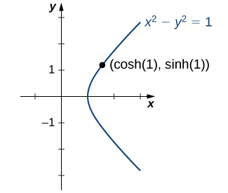
Figure 7. The unit hyperbola [latex]\cosh^2 t-\sinh^2 t=1[/latex].
Graphs of Hyperbolic Functions
To graph [latex]\cosh x[/latex] and [latex]\sinh x[/latex], we make use of the fact that both functions approach [latex]\left(\frac{1}{2}\right)e^x[/latex] as [latex]x \to \infty[/latex], since [latex]e^{−x} \to 0[/latex] as [latex]x \to \infty[/latex]. As [latex]x \to −\infty, \, \cosh x[/latex] approaches [latex]\frac{1}{2}e^{−x}[/latex], whereas [latex]\sinh x[/latex] approaches [latex]-\frac{1}{2}e^{−x}[/latex]. Therefore, using the graphs of [latex]\frac{1}{2}e^x, \, \frac{1}{2}e^{−x}[/latex], and [latex]−\frac{1}{2}e^{−x}[/latex] as guides, we graph [latex]\cosh x[/latex] and [latex]\sinh x[/latex]. To graph [latex]\tanh x[/latex], we use the fact that [latex]\tanh(0)=0, \, -1<\tanh(x)<1[/latex] for all [latex]x, \, \tanh x \to 1[/latex] as [latex]x \to \infty[/latex], and [latex]\tanh x \to −1[/latex] as [latex]x \to −\infty[/latex]. The graphs of the other three hyperbolic functions can be sketched using the graphs of [latex]\cosh x, \, \sinh x[/latex], and [latex]\tanh x[/latex] (Figure 8).
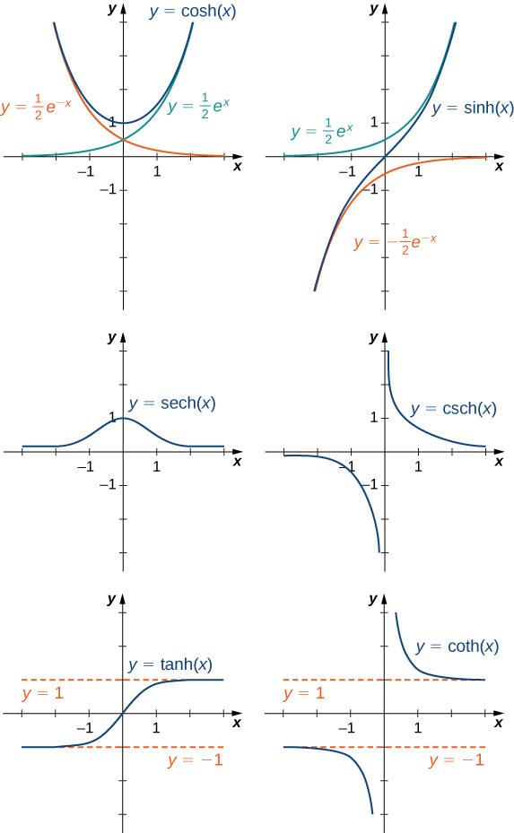
Figure 8. The hyperbolic functions involve combinations of [latex]e^x[/latex] and [latex]e^{−x}[/latex].
Identities Involving Hyperbolic Functions
The identity [latex]\cosh^2 t-\sinh^2 t[/latex], shown in Figure 7, is one of several identities involving the hyperbolic functions, some of which are listed next. The first four properties follow easily from the definitions of hyperbolic sine and hyperbolic cosine. Except for some differences in signs, most of these properties are analogous to identities for trigonometric functions.
Identities Involving Hyperbolic Functions
- [latex]\cosh(−x)=\cosh x[/latex]
- [latex]\sinh(−x)=−\sinh x[/latex]
- [latex]\cosh x+\sinh x=e^x[/latex]
- [latex]\cosh x-\sinh x=e^{−x}[/latex]
- [latex]\cosh^2 x-\sinh^2 x=1[/latex]
- [latex]1-\tanh^2 x=\text{sech}^2 x[/latex]
- [latex]\coth^2 x-1=\text{csch}^2 x[/latex]
- [latex]\sinh(x \pm y)=\sinh x \cosh y \pm \cosh x \sinh y[/latex]
- [latex]\cosh (x \pm y)=\cosh x \cosh y \pm \sinh x \sinh y[/latex]
Example: Evaluating Hyperbolic Functions
- Simplify [latex]\sinh(5 \ln x)[/latex].
- If [latex]\sinh x=\frac{3}{4}[/latex], find the values of the remaining five hyperbolic functions.
Watch the following video to see the worked solution to Example: Evaluating Hyperbolic Functions
Try It
Simplify [latex]\cosh(2 \ln x)[/latex].
Inverse Hyperbolic Functions
From the graphs of the hyperbolic functions, we see that all of them are one-to-one except [latex]\cosh x[/latex] and [latex]\text{sech} \, x[/latex]. If we restrict the domains of these two functions to the interval [latex][0,\infty)[/latex], then all the hyperbolic functions are one-to-one, and we can define the inverse hyperbolic functions. Since the hyperbolic functions themselves involve exponential functions, the inverse hyperbolic functions involve logarithmic functions.
Definition
Inverse Hyperbolic Functions:
Let’s look at how to derive the first equation. The others follow similarly. Suppose [latex]y=\sinh^{-1} x[/latex]. Then, [latex]x=\sinh y[/latex] and, by the definition of the hyperbolic sine function, [latex]x=\frac{e^y-e^{−y}}{2}[/latex]. Therefore,
Multiplying this equation by [latex]e^y[/latex], we obtain
This can be solved like a quadratic equation, with the solution
Since [latex]e^y>0[/latex], the only solution is the one with the positive sign. Applying the natural logarithm to both sides of the equation, we conclude that
Example: Evaluating Inverse Hyperbolic Functions
Evaluate each of the following expressions
[latex]\sinh^{-1}(2)[/latex]
[latex]\tanh^{-1}\left(\frac{1}{4}\right)[/latex]
Try It
Evaluate [latex]\tanh^{-1}\left(\frac{1}{2}\right)[/latex].
Candela Citations
- 1.5 Exponential and Logarithmic Functions. License: CC BY: Attribution
- Calculus Volume 1. Authored by: Gilbert Strang, Edwin (Jed) Herman. Provided by: OpenStax. Located at: https://openstax.org/details/books/calculus-volume-1. License: CC BY-NC-SA: Attribution-NonCommercial-ShareAlike. License Terms: Access for free at https://openstax.org/books/calculus-volume-1/pages/1-introduction
