Using correct notation, describe an infinite limit
Define a vertical asymptote
Evaluating the limit of a function at a point or evaluating the limit of a function from the right and left at a point helps us to characterize the behavior of a function around a given value. As we shall see, we can also describe the behavior of functions that do not have finite limits.
We now turn our attention to [latex]h(x)=\frac{1}{(x-2)^2}[/latex]. From its graph we see that as the values of [latex]x[/latex] approach 2, the values of [latex]h(x)=\frac{1}{(x-2)^2}[/latex] become larger and larger and, in fact, become infinite. Mathematically, we say that the limit of [latex]h(x)[/latex] as [latex]x[/latex] approaches 2 is positive infinity. Symbolically, we express this idea as
More generally, we define infinite limits as follows:
Definition
We define three types of infinite limits.
Infinite limits from the left: Let [latex]f(x)[/latex] be a function defined at all values in an open interval of the form [latex](b,a)[/latex].
If the values of [latex]f(x)[/latex] increase without bound as the values of [latex]x[/latex] (where [latex]x[latex]\underset{x\to a^-}{\lim}f(x)=+\infty[/latex].
If the values of [latex]f(x)[/latex] decrease without bound as the values of [latex]x[/latex] (where [latex]x[latex]\underset{x\to a^-}{\lim}f(x)=−\infty[/latex].
Infinite limits from the right: Let [latex]f(x)[/latex] be a function defined at all values in an open interval of the form [latex](a,c)[/latex].
If the values of [latex]f(x)[/latex] increase without bound as the values of [latex]x[/latex] (where [latex]x>a[/latex]) approach the number [latex]a[/latex], then we say that the limit as [latex]x[/latex] approaches [latex]a[/latex] from the right is positive infinity and we write
If the values of [latex]f(x)[/latex] decrease without bound as the values of [latex]x[/latex] (where [latex]x>a[/latex]) approach the number [latex]a[/latex], then we say that the limit as [latex]x[/latex] approaches [latex]a[/latex] from the right is negative infinity and we write
Two-sided infinite limit: Let [latex]f(x)[/latex] be defined for all [latex]x\ne a[/latex] in an open interval containing [latex]a[/latex].
If the values of [latex]f(x)[/latex] increase without bound as the values of [latex]x[/latex] (where [latex]x\ne a[/latex]) approach the number [latex]a[/latex], then we say that the limit as [latex]x[/latex] approaches [latex]a[/latex] is positive infinity and we write
If the values of [latex]f(x)[/latex] decrease without bound as the values of [latex]x[/latex] (where [latex]x\ne a[/latex]) approach the number [latex]a[/latex], then we say that the limit as [latex]x[/latex] approaches [latex]a[/latex] is negative infinity and we write
It is important to understand that when we write statements such as [latex]\underset{x\to a}{\lim}f(x)=+\infty[/latex] or [latex]\underset{x\to a}{\lim}f(x)=−\infty[/latex] we are describing the behavior of the function, as we have just defined it. We are not asserting that a limit exists. For the limit of a function [latex]f(x)[/latex] to exist at [latex]a[/latex], it must approach a real number [latex]L[/latex] as [latex]x[/latex] approaches [latex]a[/latex]. That said, if, for example, [latex]\underset{x\to a}{\lim}f(x)=+\infty[/latex], we always write [latex]\underset{x\to a}{\lim}f(x)=+\infty[/latex] rather than [latex]\underset{x\to a}{\lim}f(x)[/latex] DNE.
Example: Recognizing an Infinite Limit
Evaluate each of the following limits, if possible. Use a table of functional values and graph [latex]f(x)=1/x[/latex] to confirm your conclusion.
Since [latex]\underset{x\to 0^-}{\lim}\frac{1}{x}=−\infty[/latex] and [latex]\underset{x\to 0^+}{\lim}\frac{1}{x}=+\infty[/latex] have different values, we conclude that
The graph of [latex]f(x)=\frac{1}{x}[/latex] in Figure 8 confirms these conclusions.
Figure 8. The graph of [latex]f(x)=\frac{1}{x}[/latex] confirms that the limit as [latex]x[/latex] approaches 0 does not exist.
Try It
Evaluate each of the following limits, if possible. Use a table of functional values and graph [latex]f(x)=\dfrac{1}{x^2}[/latex] to confirm your conclusion.
a. [latex]\underset{x\to 0^-}{\lim}\frac{1}{x^2}=+\infty[/latex];
b. [latex]\underset{x\to 0^+}{\lim}\frac{1}{x^2}=+\infty[/latex];
c. [latex]\underset{x\to 0}{\lim}\frac{1}{x^2}=+\infty[/latex]
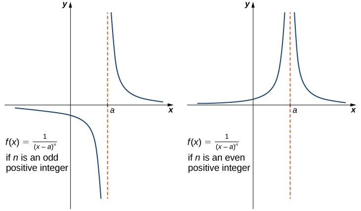
It is useful to point out that functions of the form [latex]f(x)=\dfrac{1}{(x-a)^n}[/latex], where [latex]n[/latex] is a positive integer, have infinite limits as [latex]x[/latex] approaches [latex]a[/latex] from either the left or right (Figure 9). These limits are summarized below the graphs.
Figure 9. The function [latex]f(x)=1/(x-a)^n[/latex] has infinite limits at [latex]a[/latex].
Infinite Limits from Positive Integers
If [latex]n[/latex] is a positive even integer, then
We should also point out that in the graphs of [latex]f(x)=\dfrac{1}{(x-a)^n}[/latex], points on the graph having [latex]x[/latex]-coordinates very near to [latex]a[/latex] are very close to the vertical line [latex]x=a[/latex]. That is, as [latex]x[/latex] approaches [latex]a[/latex], the points on the graph of [latex]f(x)[/latex] are closer to the line [latex]x=a[/latex]. The line [latex]x=a[/latex] is called a vertical asymptote of the graph. We formally define a vertical asymptote as follows:
Definition
Let [latex]f(x)[/latex] be a function. If any of the following conditions hold, then the line [latex]x=a[/latex] is a vertical asymptote of [latex]f(x)[/latex]:
Evaluate each of the following limits using the limits summarized under Figure 9. Identify any vertical asymptotes of the function [latex]f(x)=\dfrac{1}{(x+3)^4}[/latex].
The function [latex]f(x)=\frac{1}{(x+3)^4}[/latex] has a vertical asymptote of [latex]x=-3[/latex].
Watch the following video to see the more examples of finding a vertical asymptote.
Closed Captioning and Transcript Information for Video
For closed captioning, open the video on its original page by clicking the Youtube logo in the lower right-hand corner of the video display. In YouTube, the video will begin at the same starting point as this clip, but will continue playing until the very end.
a. [latex]\underset{x\to 2^-}{\lim}\frac{1}{(x-2)^3}=−\infty[/latex];
b. [latex]\underset{x\to 2^+}{\lim}\frac{1}{(x-2)^3}=+\infty[/latex];
c. [latex]\underset{x\to 2}{\lim}\frac{1}{(x-2)^3}[/latex] DNE. The line [latex]x=2[/latex] is the vertical asymptote of [latex]f(x)=\frac{1}{(x-2)^3}[/latex].
In the next example, we put our knowledge of various types of limits to use to analyze the behavior of a function at several different points.
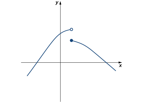
Example: Behavior of a Function at Different Points
Use the graph of [latex]f(x)[/latex] in Figure 10 to determine each of the following values:
Watch the following video to see the worked solution to Example: Behavior of a Function at Different Points. Note this video also repeats the steps for x = 3.
Closed Captioning and Transcript Information for Video
For closed captioning, open the video on its original page by clicking the Youtube logo in the lower right-hand corner of the video display. In YouTube, the video will begin at the same starting point as this clip, but will continue playing until the very end.

![The graph of a function f(x) described by the above limits and values. There is a smooth curve for values below x=-2; at (-2, 3), there is an open circle. There is a smooth curve between (-2, 1] with a closed circle at (1,6). There is an open circle at (1,3), and a smooth curve stretching from there down asymptotically to negative infinity along x=3. The function also curves asymptotically along x=3 on the other side, also stretching to negative infinity. The function then changes concavity in the first quadrant around y=4.5 and continues up.](https://s3-us-west-2.amazonaws.com/courses-images/wp-content/uploads/sites/2332/2018/01/11202918/CNX_Calc_Figure_02_02_015.jpg)