Learning Outcomes
- Evaluate inverse trigonometric functions
The six basic trigonometric functions are periodic, and therefore they are not one-to-one. However, if we restrict the domain of a trigonometric function to an interval where it is one-to-one, we can define its inverse. Consider the sine function. The sine function is one-to-one on an infinite number of intervals, but the standard convention is to restrict the domain to the interval [latex][-\frac{\pi}{2},\frac{\pi}{2}][/latex]. By doing so, we define the inverse sine function on the domain [latex][-1,1][/latex] such that for any [latex]x[/latex] in the interval [latex][-1,1][/latex], the inverse sine function tells us which angle [latex]\theta[/latex] in the interval [latex][-\frac{\pi}{2},\frac{\pi}{2}][/latex] satisfies [latex]\sin \theta =x[/latex]. Similarly, we can restrict the domains of the other trigonometric functions to define inverse trigonometric functions, which are functions that tell us which angle in a certain interval has a specified trigonometric value.
Definition
The inverse sine function, denoted [latex]\sin^{-1}[/latex] or arcsin, and the inverse cosine function, denoted [latex]\cos^{-1}[/latex] or arccos, are defined on the domain [latex]D=\{x|-1 \le x \le 1\}[/latex] as follows:
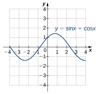
The inverse tangent function, denoted [latex]\tan^{-1}[/latex] or arctan, and inverse cotangent function, denoted [latex]\cot^{-1}[/latex] or arccot, are defined on the domain [latex]D=\{x|-\infty The inverse cosecant function, denoted [latex]\csc^{-1}[/latex] or arccsc, and inverse secant function, denoted [latex]\sec^{-1}[/latex] or arcsec, are defined on the domain [latex]D=\{x| \, |x| \ge 1\}[/latex] as follows: To graph the inverse trigonometric functions, we use the graphs of the trigonometric functions restricted to the domains defined earlier and reflect the graphs about the line [latex]y=x[/latex] (Figure 16). Figure 16. The graph of each of the inverse trigonometric functions is a reflection about the line [latex]y=x[/latex] of the corresponding restricted trigonometric function. When evaluating an inverse trigonometric function, the output is an angle. For example, to evaluate [latex]\cos^{-1}(\frac{1}{2})[/latex], we need to find an angle [latex]\theta[/latex] such that [latex]\cos \theta =\frac{1}{2}[/latex]. Clearly, many angles have this property. However, given the definition of [latex]\cos^{-1}[/latex], we need the angle [latex]\theta[/latex] that not only solves this equation, but also lies in the interval [latex][0,\pi][/latex]. We conclude that [latex]\cos^{-1}(\frac{1}{2})=\frac{\pi}{3}[/latex]. Review the following table of common sine and cosine values using reference angles, if necessary. We now consider a composition of a trigonometric function and its inverse. For example, consider the two expressions [latex]\sin (\sin^{-1}(\frac{\sqrt{2}}{2}))[/latex] and [latex]\sin^{-1}(\sin(\pi))[/latex]. For the first one, we simplify as follows: For the second one, we have The inverse function is supposed to “undo” the original function, so why isn’t [latex]\sin^{-1}(\sin (\pi))=\pi[/latex]? Recalling our definition of inverse functions, a function [latex]f[/latex] and its inverse [latex]f^{-1}[/latex] satisfy the conditions [latex]f(f^{-1}(y))=y[/latex] for all [latex]y[/latex] in the domain of [latex]f^{-1}[/latex] and [latex]f^{-1}(f(x))=x[/latex] for all [latex]x[/latex] in the domain of [latex]f[/latex], so what happened here? The issue is that the inverse sine function, [latex]\sin^{-1}[/latex], is the inverse of the restricted sine function defined on the domain [latex][-\frac{\pi}{2},\frac{\pi}{2}][/latex]. Therefore, for [latex]x[/latex] in the interval [latex][-\frac{\pi}{2},\frac{\pi}{2}][/latex], it is true that [latex]\sin^{-1}(\sin x)=x[/latex]. However, for values of [latex]x[/latex] outside this interval, the equation does not hold, even though [latex]\sin^{-1}(\sin x)[/latex] is defined for all real numbers [latex]x[/latex]. What about [latex]\sin (\sin^{-1}y)[/latex]? Does that have a similar issue? The answer is no. Since the domain of [latex]\sin^{-1}[/latex] is the interval [latex][-1,1][/latex], we conclude that [latex]\sin (\sin^{-1}y)=y[/latex] if [latex]-1 \le y \le 1[/latex] and the expression is not defined for other values of [latex]y[/latex]. To summarize, and Similarly, for the cosine function, and Similar properties hold for the other trigonometric functions and their inverses. Evaluate each of the following expressions. Watch the following video to see the worked solution to Example: Evaluating Expressions Involving Inverse Trigonometric Functions In many areas of science, engineering, and mathematics, it is useful to know the maximum value a function can obtain, even if we don’t know its exact value at a given instant. For instance, if we have a function describing the strength of a roof beam, we would want to know the maximum weight the beam can support without breaking. If we have a function that describes the speed of a train, we would want to know its maximum speed before it jumps off the rails. Safe design often depends on knowing maximum values. This project describes a simple example of a function with a maximum value that depends on two equation coefficients. We will see that maximum values can depend on several factors other than the independent variable [latex]x[/latex]. Figure 17. The graph of [latex]y= \sin x + \cos x[/latex]. Using a graphing calculator or other graphing device, estimate the [latex]x[/latex]– and [latex]y[/latex]-values of the maximum point for the graph (the first such point where [latex]x>0[/latex]). It may be helpful to express the [latex]x[/latex]-value as a multiple of [latex]\pi[/latex].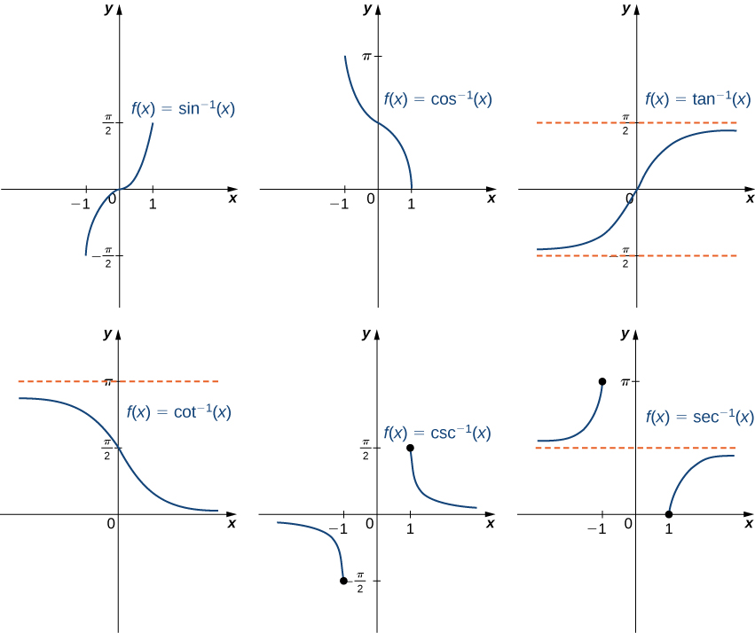
Recall: Commonly encountered angles in first quadrant of the unit circle
Angle
0
[latex]\frac{\pi }{6}[/latex], or 30°
[latex]\frac{\pi }{4}[/latex], or 45°
[latex]\frac{\pi }{3}[/latex], or 60°
[latex]\frac{\pi }{2}[/latex], or 90°
Cosine
1
[latex]\frac{\sqrt{3}}{2}[/latex]
[latex]\frac{\sqrt{2}}{2}[/latex]
[latex]\frac{1}{2}[/latex]
0
Sine
0
[latex]\frac{1}{2}[/latex]
[latex]\frac{\sqrt{2}}{2}[/latex]
[latex]\frac{\sqrt{3}}{2}[/latex]
1
Example: Evaluating Expressions Involving Inverse Trigonometric Functions
Activity: The Maximum Value of a Function
[latex]A[/latex]
[latex]B[/latex]
[latex]x[/latex]
[latex]y[/latex]
[latex]A[/latex]
[latex]B[/latex]
[latex]x[/latex]
[latex]y[/latex]
0
1
[latex]\sqrt{3}[/latex]
1
1
0
1
[latex]\sqrt{3}[/latex]
1
1
12
5
1
2
5
12
2
1
2
2
3
4
4
3
Try It
Candela Citations
