Learning Outcomes
- Recognize the degree of a polynomial
- Find the roots of a quadratic polynomial
- Describe the graphs of basic odd and even polynomial functions
A linear function is a special type of a more general class of functions: polynomials. A polynomial function is any function that can be written in the form
for some integer [latex]n\ge 0[/latex] and constants [latex]a_n, \, a_{n-1}, \cdots, a_0[/latex], where [latex]a_n\ne 0[/latex].
In the case when [latex]n=0[/latex], we allow for [latex]a_0=0[/latex]; if [latex]a_0=0[/latex], the function [latex]f(x)=0[/latex] is called the zero function. The value [latex]n[/latex] is called the degree of the polynomial; the constant [latex]a_n[/latex] is called the leading coefficient. A linear function of the form [latex]f(x)=mx+b[/latex] is a polynomial of degree 1 if [latex]m\ne 0[/latex] and degree 0 if [latex]m=0[/latex]. A polynomial of degree 0 is also called a constant function. A polynomial function of degree 2 is called a quadratic function. In particular, a quadratic function has the form [latex]f(x)=ax^2+bx+c[/latex], where [latex]a\ne 0[/latex]. A polynomial function of degree 3 is called a cubic function.
Try It
Power Functions
Some polynomial functions are power functions. A power function is any function of the form [latex]f(x)=ax^b[/latex], where [latex]a[/latex] and [latex]b[/latex] are any real numbers. The exponent in a power function can be any real number, but here we consider the case when the exponent is a positive integer. (We consider other cases later.) If the exponent is a positive integer, then [latex]f(x)=ax^n[/latex] is a polynomial. If [latex]n[/latex] is even, then [latex]f(x)=ax^n[/latex] is an even function because [latex]f(−x)=a(−x)^n=ax^n[/latex] if [latex]n[/latex] is even. If [latex]n[/latex] is odd, then [latex]f(x)=ax^n[/latex] is an odd function because [latex]f(−x)=a(−x)^n=−ax^n[/latex] if [latex]n[/latex] is odd (Figure 5).
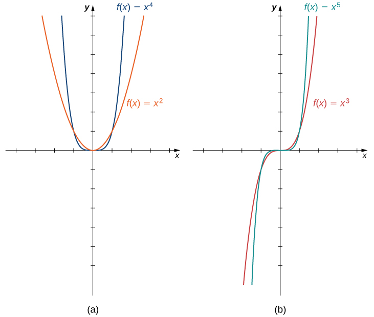
Figure 5. (a) For any even integer [latex]n,f(x)=ax^n[/latex] is an even function. (b) For any odd integer [latex]n,f(x)=ax^n[/latex] is an odd function.
Behavior at Infinity
To determine the behavior of a function [latex]f[/latex] as the inputs approach infinity, we look at the values [latex]f(x)[/latex] as the inputs, [latex]x[/latex], become larger. For some functions, the values of [latex]f(x)[/latex] approach a finite number. For example, for the function [latex]f(x)=2+\frac{1}{x}[/latex], the values [latex]\frac{1}{x}[/latex] become closer and closer to zero for all values of [latex]x[/latex] as they get larger and larger. For this function, we say “[latex]f(x)[/latex] approaches two as [latex]x[/latex] goes to infinity,” and we write [latex]f(x)\to 2[/latex] as [latex]x\to \infty[/latex]. The line [latex]y=2[/latex] is a horizontal asymptote for the function [latex]f(x)=2+\frac{1}{x}[/latex] because the graph of the function gets closer to the line as [latex]x[/latex] gets larger.
For other functions, the values [latex]f(x)[/latex] may not approach a finite number but instead may become larger for all values of [latex]x[/latex] as they get larger. In that case, we say “[latex]f(x)[/latex] approaches infinity as [latex]x[/latex] approaches infinity,” and we write [latex]f(x)\to \infty[/latex] as [latex]x\to \infty[/latex]. For example, for the function [latex]f(x)=3x^2[/latex], the outputs [latex]f(x)[/latex] become larger as the inputs [latex]x[/latex] get larger. We can conclude that the function [latex]f(x)=3x^2[/latex] approaches infinity as [latex]x[/latex] approaches infinity, and we write [latex]3x^2\to \infty[/latex] as [latex]x\to \infty[/latex]. The behavior as [latex]x \to −\infty[/latex] and the meaning of [latex]f(x) \to −\infty[/latex] as [latex]x \to \infty[/latex] or [latex]x \to −\infty[/latex] can be defined similarly. We can describe what happens to the values of [latex]f(x)[/latex] as [latex]x \to \infty[/latex] and as [latex]x \to −\infty[/latex] as the end behavior of the function.
To understand the end behavior for polynomial functions, we can focus on quadratic and cubic functions. The behavior for higher-degree polynomials can be analyzed similarly. Consider a quadratic function [latex]f(x)=ax^2+bx+c[/latex]. If [latex]a>0[/latex], the values [latex]f(x) \to \infty[/latex] as [latex]x \to \pm \infty[/latex]. If [latex]a<0[/latex], the values [latex]f(x) \to −\infty[/latex] as [latex]x \to \pm \infty[/latex]. Since the graph of a quadratic function is a parabola, the parabola opens upward if [latex]a>0[/latex]; the parabola opens downward if [latex]a<0[/latex]. (See Figure 6(a).)
Now consider a cubic function [latex]f(x)=ax^3+bx^2+cx+d[/latex]. If [latex]a>0[/latex], then [latex]f(x) \to \infty[/latex] as [latex]x \to \infty[/latex] and [latex]f(x) \to -\infty[/latex] as [latex]x \to −\infty[/latex]. If [latex]a<0[/latex], then [latex]f(x) \to −\infty[/latex] as [latex]x \to \infty[/latex] and [latex]f(x) \to \infty[/latex] as [latex]x \to −\infty[/latex]. As we can see from both of these graphs, the leading term of the polynomial determines the end behavior. (See Figure 6(b).)
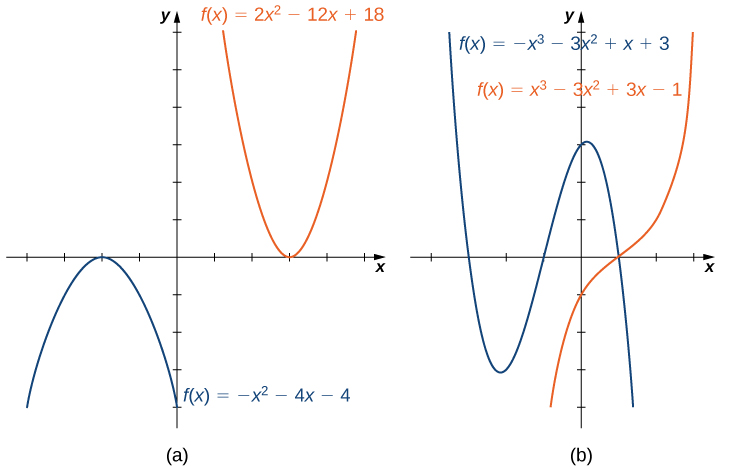
Figure 6. (a) For a quadratic function, if the leading coefficient [latex]a>0[/latex], the parabola opens upward. If [latex]a<0[/latex], the parabola opens downward. (b) For a cubic function [latex]f[/latex], if the leading coefficient [latex]a>0[/latex], the values [latex]f(x) \to \infty [/latex] as [latex]x\to \infty [/latex] and the values [latex]f(x)\to −\infty[/latex] as [latex]x \to −\infty[/latex]. If the leading coefficient [latex]a<0[/latex], the opposite is true.
Zeros of Polynomial Functions
Another characteristic of the graph of a polynomial function is where it intersects the [latex]x[/latex]-axis. To determine where a function [latex]f[/latex] intersects the [latex]x[/latex]-axis, we need to solve the equation [latex]f(x)=0[/latex] for [latex]x[/latex]. In the case of the linear function [latex]f(x)=mx+b[/latex], the [latex]x[/latex]-intercept is given by solving the equation [latex]mx+b=0[/latex]. In this case, we see that the [latex]x[/latex]-intercept is given by [latex](−\frac{b}{m},0)[/latex]. In the case of a quadratic function, finding the [latex]x[/latex]-intercept(s) requires finding the zeros of a quadratic equation: [latex]ax^2+bx+c=0[/latex]. In some cases, it is easy to factor the polynomial [latex]ax^2+bx+c[/latex] to find the zeros. If not, we make use of the quadratic formula.
The Quadratic Formula
Consider the quadratic equation
where [latex]a\ne 0[/latex]. The solutions of this equation are given by the quadratic formula
If the discriminant [latex]b^2-4ac>0[/latex], this formula tells us there are two real numbers that satisfy the quadratic equation. If [latex]b^2-4ac=0[/latex], this formula tells us there is only one solution, and it is a real number. If [latex]b^2-4ac<0[/latex], no real numbers satisfy the quadratic equation.
In the case of higher-degree polynomials, it may be more complicated to determine where the graph intersects the [latex]x[/latex]-axis. In some instances, it is possible to find the [latex]x[/latex]-intercepts by factoring the polynomial to find its zeros. Remember, there are many different methods to factoring, depending on the type of polynomial.
Recall: Factoring polymonials
- The greatest common factor, or GCF, can be factored out of a polynomial. Checking for a GCF should be the first step in any factoring problem.
- Trinomials with leading coefficient 1 can be factored by finding numbers that have a product of the third term and a sum of the second term.
- Trinomials can be factored using a process called factoring by grouping.
- Perfect square trinomials and the difference of squares are special products and can be factored using equations.
- The sum of cubes and the difference of cubes can be factored using equations.
- Polynomials containing fractional and negative exponents can be factored by pulling out a GCF.
Key Equations
difference of squares [latex]{a}^{2}-{b}^{2}=\left(a+b\right)\left(a-b\right)[/latex] perfect square trinomial [latex]{a}^{2}+2ab+{b}^{2}={\left(a+b\right)}^{2}[/latex] sum of cubes [latex]{a}^{3}+{b}^{3}=\left(a+b\right)\left({a}^{2}-ab+{b}^{2}\right)[/latex] difference of cubes [latex]{a}^{3}-{b}^{3}=\left(a-b\right)\left({a}^{2}+ab+{b}^{2}\right)[/latex]
In other cases, it is impossible to calculate the exact values of the [latex]x[/latex]-intercepts. However, as we see later in the text, in cases such as this, we can use analytical tools to approximate (to a very high degree) where the [latex]x[/latex]-intercepts are located. Here we focus on the graphs of polynomials for which we can calculate their zeros explicitly.
Example: Graphing Polynomial Functions
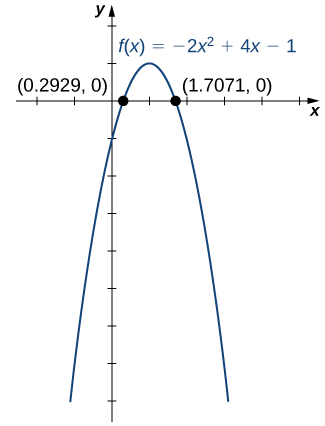
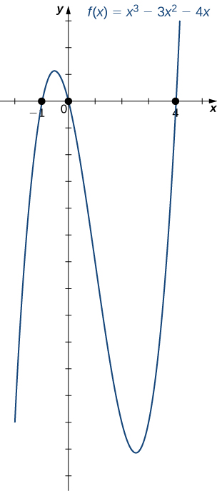
For the following functions a. and b., i. describe the behavior of [latex]f(x)[/latex] as [latex]x \to \pm \infty[/latex], ii. find all zeros of [latex]f[/latex], and iii. sketch a graph of [latex]f[/latex].
- [latex]f(x)=-2x^2+4x-1[/latex]
- [latex]f(x)=x^3-3x^2-4x[/latex]
Watch the following video to see the worked solution to Example: Graphing Polynomial Functions
Try It
Consider the quadratic function [latex]f(x)=3x^2-6x+2[/latex]. Find the zeros of [latex]f[/latex]. Does the parabola open upward or downward?
Try It
Mathematical Models (Linear and Quadratic Functions)
A large variety of real-world situations can be described using mathematical models. A mathematical model is a method of simulating real-life situations with mathematical equations. Physicists, engineers, economists, and other researchers develop models by combining observation with quantitative data to develop equations, functions, graphs, and other mathematical tools to describe the behavior of various systems accurately. Models are useful because they help predict future outcomes. Examples of mathematical models include the study of population dynamics, investigations of weather patterns, and predictions of product sales.
As an example, let’s consider a mathematical model that a company could use to describe its revenue for the sale of a particular item. The amount of revenue [latex]R[/latex] a company receives for the sale of [latex]n[/latex] items sold at a price of [latex]p[/latex] dollars per item is described by the equation [latex]R=p·n[/latex]. The company is interested in how the sales change as the price of the item changes. Suppose the data in the table below show the number of units a company sells as a function of the price per item.
| [latex]\mathbf{p}[/latex] | 6 | 8 | 10 | 12 | 14 |
| [latex]\mathbf{n}[/latex] | 19.4 | 18.5 | 16.2 | 13.8 | 12.2 |
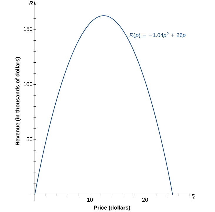
In Figure 9, we see the graph the number of units sold (in thousands) as a function of price (in dollars). We note from the shape of the graph that the number of units sold is likely a linear function of price per item, and the data can be closely approximated by the linear function [latex]n=-1.04p+26[/latex] for [latex]0\le p\le 25[/latex], where [latex]n[/latex] predicts the number of units sold in thousands. Using this linear function, the revenue (in thousands of dollars) can be estimated by the quadratic function
for [latex]0\le p\le 25[/latex]. In the example at the bottom, we use this quadratic function to predict the amount of revenue the company receives depending on the price the company charges per item. Note that we cannot conclude definitively the actual number of units sold for values of [latex]p[/latex], for which no data are collected. However, given the other data values and the graph shown, it seems reasonable that the number of units sold (in thousands) if the price charged is [latex]p[/latex] dollars may be close to the values predicted by the linear function [latex]n=-1.04p+26[/latex].
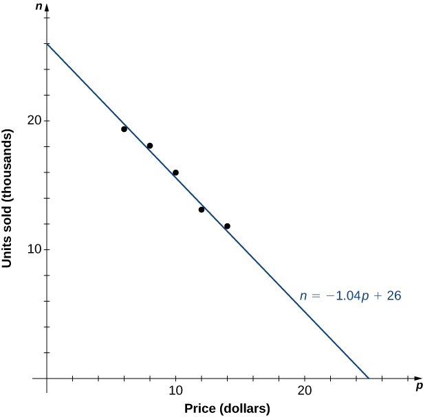
Figure 9. The data collected for the number of items sold as a function of price is roughly linear. We use the linear function [latex]n=-1.04p+26[/latex] to estimate this function.
Example: Maximizing Revenue
A company is interested in predicting the amount of revenue it will receive depending on the price it charges for a particular item. Using the data from the table earlier, the company arrives at the following quadratic function to model revenue [latex]R[/latex] as a function of price per item [latex]p[/latex]:
for [latex]0\le p\le 25[/latex].
- Predict the revenue if the company sells the item at a price of [latex]p=\$5[/latex] and [latex]p=\$17[/latex].
- Find the zeros of this function and interpret the meaning of the zeros.
- Sketch a graph of [latex]R[/latex].
- Use the graph to determine the value of [latex]p[/latex] that maximizes revenue. Find the maximum revenue.
Watch the following video to see the worked solution to Example: Maximizing Revenue
Candela Citations
- 1.2 Basic Classes of Functions. Authored by: Ryan Melton. License: CC BY: Attribution
- Calculus Volume 1. Authored by: Gilbert Strang, Edwin (Jed) Herman. Provided by: OpenStax. Located at: https://openstax.org/details/books/calculus-volume-1. License: CC BY-NC-SA: Attribution-NonCommercial-ShareAlike. License Terms: Access for free at https://openstax.org/books/calculus-volume-1/pages/1-introduction
