Learning Outcomes
- Describe the area problem and how it was solved by the integral
- Explain how the idea of a limit is involved in solving the area problem
- Recognize the total cost as the area under the marginal cost curve
We now turn our attention to a classic question from calculus. Many quantities in physics—for example, quantities of work—may be interpreted as the area under a curve. This leads us to ask the question: How can we find the area between the graph of a function and the [latex]x[/latex]-axis over an interval (Figure 7)?
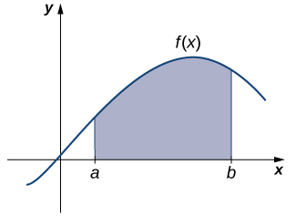
Figure 7. The Area Problem: How do we find the area of the shaded region?
As in the answer to our previous questions on velocity, we first try to approximate the solution. We approximate the area by dividing up the interval [latex][a,b][/latex] into smaller intervals in the shape of rectangles. The approximation of the area comes from adding up the areas of these rectangles (Figure 8). Recall that the area of a rectangle can be found simply by taking the length times the width.
![The graph is the same as the previous image, with one difference. Instead of the area completely shaded under the curved function, the interval [a, b] is divided into smaller intervals in the shape of rectangles. The rectangles have the same small width. The height of each rectangle is the height of the function at the midpoint of the base of that specific rectangle.](https://s3-us-west-2.amazonaws.com/courses-images/wp-content/uploads/sites/2332/2018/01/11202838/CNX_Calc_Figure_02_01_007.jpg)
Figure 8. The area of the region under the curve is approximated by summing the areas of thin rectangles.
As the widths of the rectangles become smaller (approach zero), the sums of the areas of the rectangles approach the area between the graph of [latex]f(x)[/latex] and the [latex]x[/latex]-axis over the interval [latex][a,b][/latex]. Once again, we find ourselves taking a limit. Limits of this type serve as a basis for the definition of the definite integral. Integral calculus is the study of integrals and their applications.
Example: Estimation Using Rectangles
Estimate the area between the [latex]x[/latex]-axis and the graph of [latex]f(x)=x^2+1[/latex] over the interval [latex][0,3][/latex] by using the three rectangles shown in Figure 9.
Figure 9. The area of the region under the curve of [latex]f(x)=x^2+1[/latex] can be estimated using rectangles.
Watch the following video to see the worked solution to Example: Estimation Using Rectangles
Try It
Estimate the area between the [latex]x[/latex]-axis and the graph of [latex]f(x)=x^2+1[/latex] over the interval [latex][0,3][/latex] by using the three rectangles shown here:
![A graph of the same parabola f(x) = x^2 + 1, but with a different shading strategy over the interval [0,3]. This time, the shaded rectangles are given the height of the taller corner that could intersect with the function. As such, the rectangles go higher than the height of the function.](https://s3-us-west-2.amazonaws.com/courses-images/wp-content/uploads/sites/2332/2018/01/11202843/CNX_Calc_Figure_02_01_009.jpg)
Figure 10.
Other Aspects of Calculus
So far, we have studied functions of one variable only. Such functions can be represented visually using graphs in two dimensions; however, there is no good reason to restrict our investigation to two dimensions. Suppose, for example, that instead of determining the velocity of an object moving along a coordinate axis, we want to determine the velocity of a rock fired from a catapult at a given time, or of an airplane moving in three dimensions. We might want to graph real-value functions of two variables or determine volumes of solids of the type shown in Figure 11. These are only a few of the types of questions that can be asked and answered using multivariable calculus. Informally, multivariable calculus can be characterized as the study of the calculus of functions of two or more variables. However, before exploring these and other ideas, we must first lay a foundation for the study of calculus in one variable by exploring the concept of a limit.
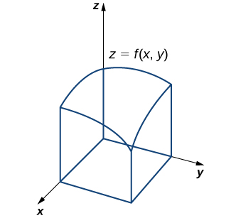
Figure 11. We can use multivariable calculus to find the volume between a surface defined by a function of two variables and a plane.
Candela Citations
- 2.1 A Preview of Calculus. Authored by: Ryan Melton. License: CC BY: Attribution
- Calculus Volume 1. Authored by: Gilbert Strang, Edwin (Jed) Herman. Provided by: OpenStax. Located at: https://openstax.org/details/books/calculus-volume-1. License: CC BY-NC-SA: Attribution-NonCommercial-ShareAlike. License Terms: Access for free at https://openstax.org/books/calculus-volume-1/pages/1-introduction
