Learning Outcomes
- Describe the tangent problem and how it led to the idea of a derivative
- Explain how the idea of a limit is involved in solving the tangent problem
- Recognize a tangent to a curve at a point as the limit of secant lines
- Identify instantaneous velocity as the limit of average velocity over a small time interval
Rate of change is one of the most critical concepts in calculus. We begin our investigation of rates of change by looking at the graphs of the three lines [latex]f(x)=-2x-3, \, g(x)=\frac{x}{2}+1[/latex], and [latex]h(x)=2[/latex], shown in Figure 1.
Figure 1. The rate of change of a linear function is constant in each of these three graphs, with the constant determined by the slope.
As we move from left to right along the graph of [latex]f(x)=-2x-3[/latex], we see that the graph decreases at a constant rate. For every 1 unit we move to the right along the [latex]x[/latex]-axis, the [latex]y[/latex]-coordinate decreases by 2 units. This rate of change is determined by the slope [latex](−2)[/latex] of the line. Similarly, the slope of [latex]\frac{1}{2}[/latex] in the function [latex]g(x)[/latex] tells us that for every change in [latex]x[/latex] of [latex]1[/latex] unit there is a corresponding change in [latex]y[/latex] of [latex]\frac{1}{2}[/latex] unit. The function [latex]h(x)=2[/latex] has a slope of zero, indicating that the values of the function remain constant. We see that the slope of each linear function indicates the rate of change of the function.
Compare the graphs of these three functions with the graph of [latex]k(x)=x^2[/latex] (Figure 2). The graph of [latex]k(x)=x^2[/latex] starts from the left by decreasing rapidly, then begins to decrease more slowly and level off, and then finally begins to increase—slowly at first, followed by an increasing rate of increase as it moves toward the right. Unlike a linear function, no single number represents the rate of change for this function. We quite naturally ask: How do we measure the rate of change of a nonlinear function?
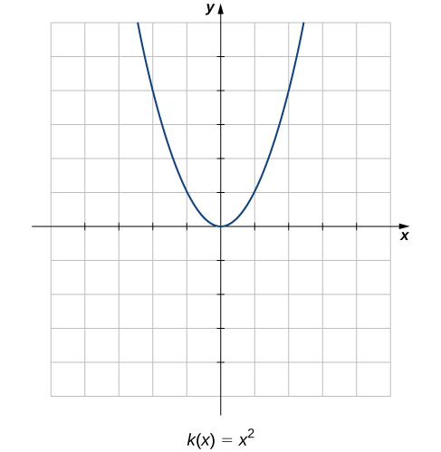
Figure 2. The function [latex]k(x)=x^2[/latex] does not have a constant rate of change.
Try It
We can approximate the rate of change of a function [latex]f(x)[/latex] at a point [latex](a,f(a))[/latex] on its graph by taking another point [latex](x,f(x))[/latex] on the graph of [latex]f(x)[/latex], drawing a line through the two points, and calculating the slope of the resulting line. Such a line is called a secant line. Figure 3 shows a secant line to a function [latex]f(x)[/latex] at a point [latex](a,f(a))[/latex].
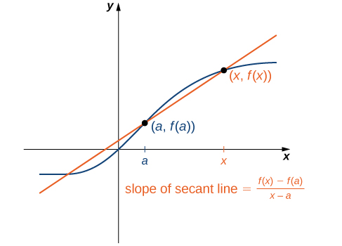
Figure 3. The slope of a secant line through a point [latex](a,f(a))[/latex] estimates the rate of change of the function at the point [latex](a,f(a))[/latex].
We formally define a secant line as follows:
Definition
The secant to the function [latex]f(x)[/latex] through the points [latex](a,f(a))[/latex] and [latex](x,f(x))[/latex] is the line passing through these points. Its slope is given by
The accuracy of approximating the rate of change of the function with a secant line depends on how close [latex]x[/latex] is to [latex]a[/latex]. As we see in Figure 4, if [latex]x[/latex] is closer to [latex]a[/latex], the slope of the secant line is a better measure of the rate of change of [latex]f(x)[/latex] at [latex]a[/latex].
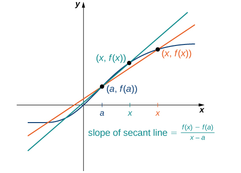
Figure 4. As x gets closer to a, the slope of the secant line becomes a better approximation to the rate of change of the function [latex]f(x)[/latex] at a.
The secant lines themselves approach a line that is called the tangent to the function [latex]f(x)[/latex] at [latex]a[/latex] (Figure 5). The slope of the tangent line to the graph at [latex]a[/latex] measures the rate of change of the function at [latex]a[/latex]. This value also represents the derivative of the function [latex]f(x)[/latex] at [latex]a[/latex], or the rate of change of the function at [latex]a[/latex]. This derivative is denoted by [latex]f^{\prime}(a)[/latex]. Differential calculus is the field of calculus concerned with the study of derivatives and their applications.
Interactive
For an interactive demonstration of the slope of a secant line that you can manipulate yourself, visit this applet from Math Insight (Note: this site requires a Java browser plugin).
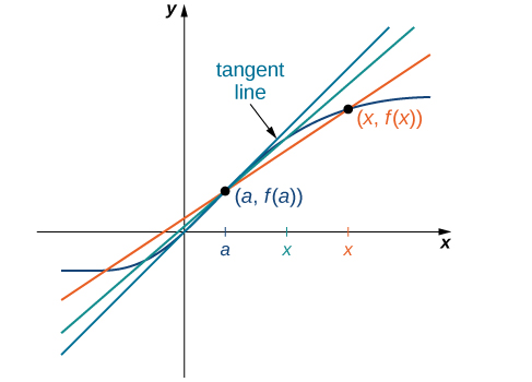
Figure 5. Solving the Tangent Problem: As x approaches a, the secant lines approach the tangent line.
Figure 5 illustrates how to find slopes of secant lines. These slopes estimate the slope of the tangent line or, equivalently, the rate of change of the function at the point at which the slopes are calculated.
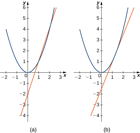
Example: Finding Slopes of Secant Lines
Estimate the slope of the tangent line (rate of change) to [latex]f(x)=x^2[/latex] at [latex]x=1[/latex] by finding slopes of secant lines through [latex](1,1)[/latex] and each of the following points on the graph of [latex]f(x)=x^2[/latex].
- [latex](2,4)[/latex]
- [latex]\left(\frac{3}{2},\frac{9}{4}\right)[/latex]
Try It
Estimate the slope of the tangent line (rate of change) to [latex]f(x)=x^2[/latex] at [latex]x=1[/latex] by finding slopes of secant lines through [latex](1,1)[/latex] and the point [latex]\left(\frac{5}{4},\frac{25}{16}\right)[/latex] on the graph of [latex]f(x)=x^2[/latex].
We continue our investigation by exploring a related question. Keeping in mind that velocity may be thought of as the rate of change of position, suppose that we have a function, [latex]s(t)[/latex], that gives the position of an object along a coordinate axis at any given time [latex]t[/latex]. Can we use these same ideas to create a reasonable definition of the instantaneous velocity at a given time [latex]t=a[/latex]? We start by approximating the instantaneous velocity with an average velocity. First, recall that the speed of an object traveling at a constant rate is the ratio of the distance traveled to the length of time it has traveled. We define the average velocity of an object over a time period to be the change in its position divided by the length of the time period.
Definition
Let [latex]s(t)[/latex] be the position of an object moving along a coordinate axis at time [latex]t[/latex]. The average velocity of the object over a time interval [latex][a,t][/latex] where [latex]a
As [latex]t[/latex] is chosen closer to [latex]a[/latex], the average velocity becomes closer to the instantaneous velocity. Note that finding the average velocity of a position function over a time interval is essentially the same as finding the slope of a secant line to a function. Furthermore, to find the slope of a tangent line at a point [latex]a[/latex], we let the [latex]x[/latex]-values approach [latex]a[/latex] in the slope of the secant line. Similarly, to find the instantaneous velocity at time [latex]a[/latex], we let the [latex]t[/latex]-values approach [latex]a[/latex] in the average velocity. This process of letting [latex]x[/latex] or [latex]t[/latex] approach [latex]a[/latex] in an expression is called taking a limit. Thus, we may define the instantaneous velocity as follows.
Definition
For a position function [latex]s(t)[/latex], the instantaneous velocity at a time [latex]t=a[/latex] is the value that the average velocities approach on intervals of the form [latex][a,t][/latex] and [latex][t,a][/latex] as the values of [latex]t[/latex] become closer to [latex]a[/latex], provided such a value exists.
The example below illustrates this concept of limits and average velocity.
Example: Finding Average Velocity
A rock is dropped from a height of 64 ft. It is determined that its height (in feet) above ground [latex]t[/latex] seconds later (for [latex]0\le t\le 2[/latex]) is given by [latex]s(t)=-16t^2+64[/latex]. Find the average velocity of the rock over each of the given time intervals. Use this information to guess the instantaneous velocity of the rock at time [latex]t=0.5[/latex].
- [latex][0.49,0.5][/latex]
- [latex][0.5,0.51][/latex]
Watch the following video to see the worked solution to Example: Finding Average Velocity
Try It
An object moves along a coordinate axis so that its position at time [latex]t[/latex] is given by [latex]s(t)=t^3[/latex]. Estimate its instantaneous velocity at time [latex]t=2[/latex] by computing its average velocity over the time interval [latex][2,2.001][/latex].
Candela Citations
- 2.1 A Preview of Calculus. Authored by: Ryan Melton. License: CC BY: Attribution
- Calculus Volume 1. Authored by: Gilbert Strang, Edwin (Jed) Herman. Provided by: OpenStax. Located at: https://openstax.org/details/books/calculus-volume-1. License: CC BY-NC-SA: Attribution-NonCommercial-ShareAlike. License Terms: Access for free at https://openstax.org/books/calculus-volume-1/pages/1-introduction
